Lost Secrets of the H-Bridge, Part II: Ripple Current in the DC Link Capacitor
In my last post, I talked about ripple current in inductive loads.
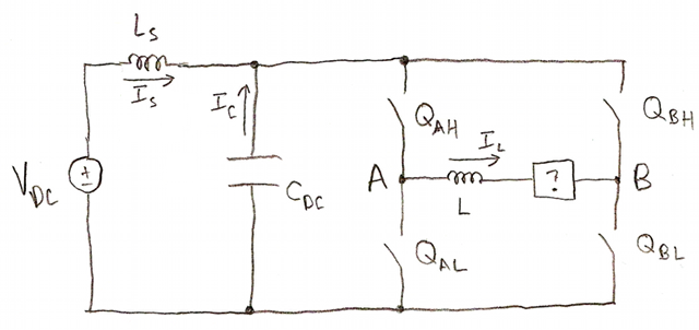
One of the assumptions we made was that the DC link was, in fact, a DC voltage source. In reality that's an approximation; no DC voltage source is perfect, and current flow will alter the DC link voltage. To analyze this, we need to go back and look at how much current actually is being drawn from the DC link. Below is an example. This is the same kind of graph as last time, except we added two things:
- nonzero DC current \( I_{Ldc} \) in the inductor
- another subplot for capacitor current
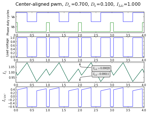
I'll give you the Python code to generate such a graph in a minute, but first let's look more closely at this. The inductor current should be familiar to you from last time, other than the DC offset, but the capacitor current is new, and kind of odd-looking, like pairs of plywood planks marching along. (At least that's what I think it looks like. :-)
We can figure out DC link capacitor current, given the inductor current and the DC supply current IS. This supply current is assumed to contain only DC and low-frequency currents, since the capacitor's role is to provide high-frequency load currents to the H-bridge. The capacitor can supply only high-frequency current; its DC current must be zero.
Note that we have drawn DC link capacitor current IC as going out of the capacitor, not in. This treats it more like a voltage source rather than a load, and will make some of this analysis more intuitive, although we'll have to remember carefully that we've defined it this way.
There are four possibilities at any given time, depending on the state of the H-bridge switches:
- Both low-side switches QAL and QBL are on. \( I_C = - I_S \). Load current recirculates in the H-bridge and does not appear in the capacitor.
- QAH is on and QBL is on. \( I_C = I_L - I_S \).
- Both high-side switches QAH and QBH are on. \( I_C = - I_S \). Load current recirculates in the H-bridge and does not appear in the capacitor.
- QAL is on and QBH is on. \( I_C = -I_L - I_S \).
The switching pattern determines which of these states are active and for how long. Usually not all four of these states are active in a given PWM cycle. It's possible to switch this way, but it's inefficient: it doesn't make sense to put positive voltage across the load during one part of a PWM cycle and negative voltage across the load during another part. States 2 and 4 (the H bridge applying the DC link voltage across the load) are normally mutually exclusive:
If you want to put positive voltage across the load, you apply combinations of states 1, 2, and 3, and you never turn both QAL and QBH on at the same time. In this case the load current IL and the supply current IS are the same sign.

If you want to put negative voltage across the load, you apply combinations of states 1, 3, and 4, and you never turn both QAH and QBL on at the same time. In this case the load current IL and the supply current IS are opposite signs.
Center-aligned PWM will automatically generate these patterns for you.
The easiest way to summarize this, mathematically, is:
$$I_C = (s_A - s_B) I_L - I_S$$
where sA and sB are the switching functions of nodes A and B: 1 if the high-side switch is on, 0 if the low-side switch is on.
Finally, because this current flows out of a capacitor, that requires its average value to be zero, and therefore \( I_S = (D_A - D_B) I_L = DI_L \), where DA and DB are the half-bridge duty cycles, and \( D = D_A - D_B \) is the effective duty cycle across the load.
So let's bring up our Python PWM simulation again and generate these graphs. (For those of you reading this as an IPython notebook, make sure you run the following cells. If you're reading this as a blog post, skip ahead. If you're allergic to math and you really can't stomach lots of graphs and algebra, I apologize, and maybe you should just skip to the summary.)
import matplotlib.pyplot as plt
import numpy as np
import scipy.integrate

def ramp(t): return t % 1
def sawtooth(t): return 1-abs(2*(t % 1) - 1)

def pwm(t,D,centeralign = False):
  '''generate PWM signals with duty cycle D'''
  return ((sawtooth(t) if centeralign else ramp(t)) <= D) * 1.0

def rms(t,y):
    return np.sqrt(np.trapz(y*y,t)/(np.amax(t)-np.amin(t)))

def digitalplotter(t,*signals):
  '''return a plotting function that takes an axis and plots
digital signals (or other signals in the 0-1 range)'''
  def f(ax):
    n = len(signals)
    for (i,sig) in enumerate(signals):
      ofs = (n-1-i)*1.1
      plotargs = []
      for y in sig[1:]:
        if isinstance(y,basestring):
          plotargs += [y]
        else:
          plotargs += [t,y+ofs]
      ax.plot(*plotargs)
    ax.set_yticks((n-1-np.arange(n))*1.1+0.55)
    ax.set_yticklabels([sig[0] for sig in signals])
    ax.set_ylim(-0.1,n*1.1)
  return f

def extendrange(ra,rb):
  '''return a tuple (x1,x2) representing the interval from x1 to x2,
given two input ranges of the same form, or None (representing no input).'''
  if ra is None:
    return rb
  elif rb is None:
    return ra
  else:
    return (min(ra[0],rb[0]),max(ra[1],rb[1]))

def createLimits(margin, *args):
    '''add proportional margin to an interval:
createLimits(0.1, (1,3),(2,4),(0,2)) calculates the maximum extent
of the ranges provided, in this case (0,4), and adds another 0.1 (10%)
to the extent symmetrically, thus returning (-0.2, 4.2).'''
    r = None
    for x in args:
        r = extendrange(r, (np.min(x),np.max(x)))
    rmargin = (r[1]-r[0])*margin/2.0
    return (r[0]-rmargin,r[1]+rmargin)

def calcripple(t,y):
    ''' calculate ripple current by integrating the input,
then adjusting it by a linear function to put both endpoints
at the same value. The slope of the linear function is the
mean value of the input; the offset is chosen to make the mean value
of the output ripple current = 0.'''
    T = t[-1]-t[0]
    yint0 = np.append([0],scipy.integrate.cumtrapz(y,t))
    # cumtrapz produces a vector of length N-1
    # so we need to add one element back in at the beginning
    meanval0 = yint0[-1]/T
    yint1 = yint0 - (t-t[0])*meanval0
    meanval1 = scipy.integrate.trapz(yint1,t)/T
    return yint1 - meanval1

def annotate_level(ax,t,yline,ytext,text,style='k:'):
    tlim = [min(t),max(t)]
    tannot0 = tlim[0] + (tlim[1]-tlim[0])*0.5
    tannot1 = tlim[0] + (tlim[1]-tlim[0])*0.6
    ax.plot(tlim,[yline]*2,style)
    # see:
    # http://matplotlib.org/api/axes_api.html#matplotlib.axes.Axes.annotate
    ax.annotate(text, xy=(tannot0,yline), xytext=(tannot1,ytext),
        bbox=dict(boxstyle="round", fc="0.9"),
        arrowprops=dict(arrowstyle="->",
          connectionstyle="arc,angleA=0,armA=20,angleB=%d,armB=15,rad=7"
             % (-90 if ytext < yline else 90)))

def annotate_ripple(ax,t,Iab,I_Ldc):
    # annotate with peak values
    for y in [min(Iab),max(Iab)]:
      yofs = y-I_Ldc
      annotate_level(ax,t,y,yofs*0.3 + I_Ldc, '$I_{Ldc} %+.5f$' % yofs)


def showripple(fig,t,Va,Vb,I_Ldc,titlestring):
    '''plot ripple current as well as phase duty cycles and load voltage'''
    axlist = []
    Iabripple = calcripple(t,Va-Vb)
    Iab = Iabripple + I_Ldc
    margin = 0.1
    ax = fig.add_subplot(3,1,1)
    digitalplotter(t,('Va',Va),('Vb',Vb))(ax)
    ax.set_ylabel('Phase duty cycles')
    axlist.append(ax)

    ax = fig.add_subplot(3,1,2)
    ax.plot(t,Va-Vb)
    ax.set_ylim(createLimits(margin,Va-Vb))
    ax.set_ylabel('Load voltage')
    axlist.append(ax)

    ax = fig.add_subplot(3,1,3)
    ax.plot(t,Iab)
    ax.set_ylim(createLimits(margin,Iab))
    ax.set_ylabel('Load current')
    axlist.append(ax)
    annotate_ripple(ax,t,Iab,I_Ldc)

    fig.suptitle(titlestring, fontsize=16)
    return axlist

def showpwmripple(fig,t,Da,Db,I_Ldc,centeralign=False):
    return showripple(fig,t,
               pwm(t,Da,centeralign),
               pwm(t,Db,centeralign),
               I_Ldc,
               titlestring='%s-aligned pwm, $D_a$=%.3f, $D_b$=%.3f, $I_{Ldc}$=%.3f' %
                 ('Center' if centeralign else 'Edge', Da, Db, I_Ldc))
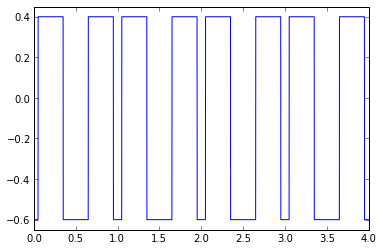
Okay! Now let's just make sure we can run this, to show ripple current in the load inductance. Remember, we're normalizing ripple current to \( I_{R0} = VT/L \).
t = np.arange(0,4,0.0005)
fig = plt.figure(figsize=(8, 6), dpi=80)
showpwmripple(fig, t, 0.7, 0.1, I_Ldc=1, centeralign=True)
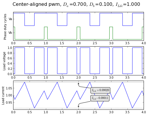
Now we have to figure out DC link capacitor current, given the inductor current. As I mentioned earlier,
$$I_{CDC} = (s_A - s_B) I_L - I_S$$
where sA and sB are the switching functions of nodes A and B: 1 if the high-side switch is on, 0 if the low-side switch is on.
Let's write some Python to simulate this, given what we know so far:
def calc_capacitor_ripple(pwmA,pwmB,I_L,I_S):
    return (pwmA-pwmB)*I_L - I_S
That's it! Really! Now let's add this to our PWM graph:
def showripple2(fig,t,pwmA,pwmB,I_Ldc,I_S,titlestring=''):
    '''plot ripple current in inductor and capacitor
as well as phase duty cycles and load voltage'''
    axlist = []
    Iabripple = calcripple(t,pwmA-pwmB)
    Iab = Iabripple + I_Ldc
    Icdc = calc_capacitor_ripple(pwmA,pwmB,Iab,I_S)

    margin = 0.1
    ax = fig.add_subplot(4,1,1)
    digitalplotter(t,('Va',pwmA),('Vb',pwmB))(ax)
    ax.set_ylabel('Phase duty cycles')
    axlist.append(ax)

    ax = fig.add_subplot(4,1,2)
    ax.plot(t,pwmA-pwmB)
    ax.set_ylim(createLimits(margin,pwmA-pwmB))
    ax.set_ylabel('Load voltage')
    axlist.append(ax)

    ax = fig.add_subplot(4,1,3)
    ax.plot(t,Iab)
    ax.set_ylim(createLimits(margin,Iab))
    ax.set_ylabel('Ripple current')
    axlist.append(ax)

    ax = fig.add_subplot(4,1,3)
    ax.plot(t,Iab)
    ax.set_ylim(createLimits(margin,Iab))
    ax.set_ylabel('$I_L$',fontsize=14)
    axlist.append(ax)
    annotate_ripple(ax,t,Iab,I_Ldc)

    ax = fig.add_subplot(4,1,4)
    ax.plot(t,Icdc)
    ax.set_ylim(createLimits(margin,Icdc))
    ax.set_ylabel('$I_{CDC}$',fontsize=14)
    axlist.append(ax)

    fig.suptitle(titlestring, fontsize=16)

    return axlist

def showpwmripple2(fig,t,Da,Db,I_Ldc,centeralign=False):
    return showripple2(fig,t,
               pwm(t,Da,centeralign),
               pwm(t,Db,centeralign),
               I_Ldc,
               (Da-Db)*I_Ldc,
               titlestring='%s-aligned pwm, $D_a$=%.3f, $D_b$=%.3f, $I_{Ldc}$=%.3f' %
                 ('Center' if centeralign else 'Edge', Da, Db, I_Ldc))
fig = plt.figure(figsize=(8, 6), dpi=80)
showpwmripple2(fig, t, 0.1, 0.7, I_Ldc=1.0, centeralign=True)
fig = plt.figure(figsize=(8, 6), dpi=80)
showpwmripple2(fig, t, 0.7, 0.1, I_Ldc=1.0, centeralign=True)
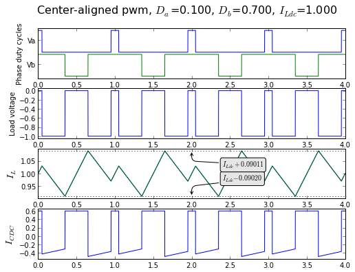
That wasn't so hard! Now we can simulate any situation where we know Da, Db, and ILdc. The symbolic analysis is a bit tricky (and grungy), so let's divide and conquer.
Superposition
Superposition is a very powerful tool. It's a way of understanding linear systems by separating out pieces, analyzing the results, and then adding them back together. Linear systems allow you to do this: the response of a system to the sum of two inputs is the same as the sum of the response of the system to each input separately.
In this case, how should we divide the problem?
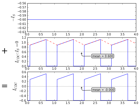
One way is to split up the capacitor current by separating out the contribution due to the DC current I_S:
def split_Icdc_1(fig, t, Da, Db, I_Ldc, centeralign=True):
    axlist = []
    pwmA = pwm(t,Da,centeralign)
    pwmB = pwm(t,Db,centeralign)
    I_S = (Da-Db)*I_Ldc
    s = np.sign(Da-Db)
    Iabripple = calcripple(t,pwmA-pwmB)
    Iab = Iabripple + I_Ldc
    Icdc = calc_capacitor_ripple(pwmA,pwmB,Iab,I_S=0)
    Icdc_mean = np.mean(Icdc)

    ax=fig.add_subplot(3,1,1)
    ax.plot(t,-I_S*ones_like(t))
    ax.set_ylabel('$-I_S$', fontsize=15)
    axlist.append(ax)

    ax=fig.add_subplot(3,1,2)
    ax.plot(t,Icdc,t,Iab*s,'--r')
    ax.set_ylabel('$I_{CDC}: I_S = 0$', fontsize=15)
    annotate_level(ax, t, Icdc_mean, np.max(Icdc)/3, 'mean = %.3f' % Icdc_mean)
    axlist.append(ax)
    fig.text(0.1,0.5,'+',fontsize=28)

    ax=fig.add_subplot(3,1,3)
    ax.plot(t,Icdc - I_S)
    ax.set_ylabel('$I_{CDC}$', fontsize=15)
    annotate_level(ax, t, Icdc_mean-I_S, (np.min(Icdc)-I_S)/3,
       'mean = %.3f' % (Icdc_mean-I_S))
    axlist.append(ax)
    fig.text(0.1,0.22,'=',fontsize=28)

    plt.subplots_adjust(left=0.25)
    return axlist

fig = plt.figure(figsize=(8, 6), dpi=80)
split_Icdc_1(fig, t, 0.7, 0.1, I_Ldc=1.0, centeralign=True)

fig = plt.figure(figsize=(8, 6), dpi=80)
split_Icdc_1(fig, t, 0.1, 0.7, I_Ldc=1.0, centeralign=True)
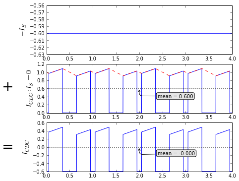
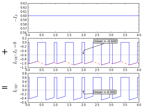
This particular split is useful for determining zero-to-peak and peak-to-peak currents. We can see pretty clearly from the middle graph that the nonzero parts of this funky waveform are equal to the current in the inductor, and we know its maximum current from the information we had last time on the inductor ripple current values. To be clear on the terminology again, we normalized to \( I_{R0} = VT/L \), and the times for nonzero capacitor ripple current are from t1 to t2, and from t4 to t5.

$$\begin{eqnarray} I_L(t_0) & = & I_L(t_3) = I_L(t_6) = 0 \cr I_L(t_1) & = & -I_L(t_5) = D \times (|D| - 2 D_0)/4 \cr I_L(t_2) & = & -I_L(t_4) = D \times (2-|D| - 2 D_0)/4 \cr D & = & D_a - D_b \cr D_0 & = & (D_a + D_b) / 2 \end{eqnarray}$$
We later figured out that
$$\max(|I_L(t_1)|,|I_L(t_2)|) = \underbrace{\frac{|D|(1-|D|)}{4}} _ {I_R/4} + \underbrace{\frac{|D| |D_0 - \tfrac{1}{2}|}{2}} _ {I_{R2}/4} $$
Also, last time, we analyzed current ripple with ILdc = 0, so we'll have to add that in:
$$\mathrm{peak}(I_L) = \frac{I_R + I_{R2}}{4} + |I_{Ldc}| $$
This is also the peak-to-peak value of Icdc. Because its waveform is asymmetric, there are two different zero-to-peak values, one positive and one negative:
$$\begin{eqnarray} \mathrm{peak_+}(I_{cdc}) & = & \frac{I_R + I_{R2}}{4} + |I_{Ldc}| - I_S = \frac{I_R + I_{R2}}{4} + |I_{Ldc}|(1-|D|) \cr \mathrm{peak_-}(I_{cdc}) & = & -I_S = -DI_{Ldc} \end{eqnarray}$$
These equations cover the case where there is positive power flow out of the H-bridge -- that is, \( I_S = DI_{Ldc} > 0 \). For regeneration, where \( I_S = DI_{Ldc} < 0 \) and power flows back into the H-bridge, the peak-to-peak current is the same, but the zero-to-peak current signs are reversed:
$$\begin{eqnarray} \mathrm{peak_+}(I_{cdc}) & = & -I_S = -DI_{Ldc} \cr \mathrm{peak_-}(I_{cdc}) & = & -\frac{I_R + I_{R2}}{4} - |I_{Ldc}| - I_S = -\frac{I_R + I_{R2}}{4} - |I_{Ldc}|(1-|D|) \end{eqnarray}$$
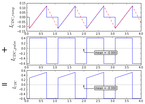
Superposition choice 2: RMS
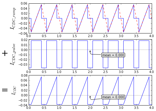
To analyze RMS current we'll choose a different separation of capacitor currents, which I'll call pulse-and-ramp:
def split_Icdc_2(fig, t, Da, Db, I_Ldc, centeralign=True):
    axlist = []
    pwmA = pwm(t,Da,centeralign)
    pwmB = pwm(t,Db,centeralign)
    I_S = (Da-Db)*I_Ldc
    s = np.sign(Da-Db)
    Iabripple = calcripple(t,pwmA-pwmB)
    Iab = Iabripple + I_Ldc
    Icdc_ramp = calc_capacitor_ripple(pwmA,pwmB,Iabripple,I_S=0)
    Icdc_pulse = I_Ldc*(pwmA-pwmB) - I_S
    Icdc = Icdc_ramp + Icdc_pulse
    Icdc_mean = np.mean(Icdc)

    ax=fig.add_subplot(3,1,1)
    ax.plot(t,Icdc_ramp,t,Iabripple*np.sign(Da-Db),'--r')
    ax.set_ylabel('$I_{CDC\_ramp}$', fontsize=18)
    axlist.append(ax)

    ax=fig.add_subplot(3,1,2)
    ax.plot(t,Icdc_pulse)
    margin = 0.1
    ylim = createLimits(margin, [-I_S,s*I_Ldc-I_S])
    ax.set_ylim(ylim)
    ax.set_ylabel('$I_{CDC\_pulse}$', fontsize=18)
    annotate_level(ax, t, mean(Icdc_pulse), ylim[0]/3, 'mean = %.3f' % mean(Icdc_pulse))
    axlist.append(ax)
    fig.text(0.1,0.5,'+',fontsize=28)

    ax=fig.add_subplot(3,1,3)
    ax.plot(t,Icdc)
    ax.set_ylabel('$I_{CDC}$', fontsize=15)
    annotate_level(ax, t, Icdc_mean, np.min(Icdc)/3, 'mean = %.3f' % (Icdc_mean))
    axlist.append(ax)
    fig.text(0.1,0.22,'=',fontsize=28)

    fig.subplots_adjust(left=0.25, right=0.95)
    return axlist

fig = plt.figure(figsize=(8, 6), dpi=80)
split_Icdc_2(fig, t, 0.7, 0.1, I_Ldc=1.0, centeralign=True)

fig2 = plt.figure(figsize=(8, 6), dpi=80)
split_Icdc_2(fig2, t, 0.1, 0.7, I_Ldc=1.0, centeralign=True)
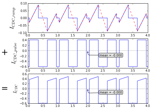

The ramp capacitor current \( I _ {CDC\_ramp} \) is the capacitor current that would result only from the inductor ripple current, and not from its DC value, so here we assume \( I _ {Ldc} \) = zero.
The pulse capacitor current \( I _ {CDC\_pulse} \) is the capacitor current that would flow with the average load current \( I _ {Ldc} \) at its real value, but with large enough inductance that the inductor ripple current were zero.
Got that? Here it is again, more concisely:
Ramp capacitor current results from inductor ripple current. It is independent of the DC inductor current.
Pulse capacitor current results from DC inductor current. It is independent of the inductor ripple current.
Why did we choose this? First, it's a little easier conceptually, since these are two different causes. More importantly, it's because the mean value of both currents is zero, and the two currents are orthogonal signals:
\( \int I _ {CDC\_ramp} I _ {CDC\_pulse} \enspace dt = 0 \)
I'm not going to prove this, but if you're clever, you can see it by noting these things:
- the ramp current is nonzero at the same times when the pulse current is nonzero
- during these two intervals, the pulse current has a constant value of \( I_{Ldc} \mathrm{sign}(D) - I_S \)
- the mean value of the ramp current is zero
OK, so they're orthogonal signals — so what? It turns out that the RMS value of the sum of orthogonal signals is the root-sum-square of each signal's RMS value. We can calculate the RMS value for each of them independently, and merge the results together into one final calculation. (This isn't true for non-orthogonal signals.)
Let's start with the ramp capacitor current.
Ramp capacitor current
Let's plot the ramp capacitor current by itself, and remember what the inductor currents are (for \( I_{Ldc} = 0 \)), to keep things fresh in our mind:
def show1period(Da,Db):
  t1period = np.arange(-0.5,1.5,0.001)
  pwmA = pwm(t1period,Da,centeralign=True)
  pwmB = pwm(t1period,Db,centeralign=True)
  fig = plt.figure()
  ax = fig.add_subplot(1,1,1)
  Iab = calcripple(t1period,pwmA-pwmB)
  Icdc_ramp = calc_capacitor_ripple(pwmA,pwmB,Iab,I_S=0)
  ax.plot(t1period,Icdc_ramp,t1period,Iab,'--r')
  ax.set_xlim(-0.1,1.1)
  ax.set_ylim(min(Iab)*1.2,max(Iab)*1.2)
  # now annotate
  (D1,D2,V) = (Db,Da,1) if Da > Db else (Da,Db,-1)
  tpts = np.array([0, D1/2, D2/2, 0.5, 1-(D2/2), 1-(D1/2), 1])
  dtpts = np.append([0],np.diff(tpts))
  vpts = np.array([0, 0, V, 0, 0, V, 0]) - (Da-Db)
  ypts = np.cumsum(vpts*dtpts)
  ax.plot(tpts,ypts,'.',markersize=8)
  for i in range(7):
    ax.annotate('$t_%d$' % i,xy=(tpts[i]+0.01,ypts[i]), fontsize=16)
  ax.legend(('$I_{CDC\\_ramp}$','$I_L$'))

show1period(0.7,0.1)
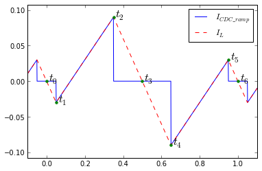
$$\begin{eqnarray} \text{with} \hspace{0.2em} I_{Ldc} & = & 0: \cr I_L(t_0) & = & I_L(t_3) = I_L(t_6) = 0 \cr I_L(t_1) & = & -I_L(t_5) = D \times (|D| - 2 D_0)/4 \cr I_L(t_2) & = & -I_L(t_4) = D \times (2-|D| - 2 D_0)/4 \cr D & = & D_a - D_b \cr D_0 & = & (D_a + D_b) / 2 \end{eqnarray}$$
The RMS of the ramp capacitor current should be less than the RMS inductor ripple current, since the waveforms are the same except that capacitor ripple current is zero outside the time intervals \( [t_1, t_2] \) and \( [t_4, t_5] \). The length of each of these intervals is just \( |D_a - D_b|/2 = |D|/2 \). We're also going to define \( D_{0dev} = D_0 - 0.5 \), which is the deviation of center-aligned PWM from the optimal common-mode duty cycle \( D_0 = 0.5 \).
import sympy
%load_ext sympy.interactive.ipythonprinting

D,D0dev,T = sympy.symbols('D D_{0dev} T')
D0 = D0dev + sympy.Integer(1)/2
def f3(y0,y1,h):
    return h*(y0*y0 + y0*y1 + y1*y1)/3
I1 = D*(abs(D)-2*D0)/4
I2 = D*(2-abs(D)-2*D0)/4
integral_squared_ripple = (f3(I1,I2,abs(D)*T/2) + f3(-I1,-I2,abs(D)*T/2))
Icdc_ramp_ms = sympy.simplify(integral_squared_ripple/T)
display('Icdc_ramp_ms=',Icdc_ramp_ms)

Icdc_ramp_ms_2 = sympy.simplify(D**2 / 48 * (12 * (D0-0.5)**2 + (abs(D)-1)**2) * abs(D))
display('Icdc_ramp_ms_2=',Icdc_ramp_ms_2)

display('difference between these=',
  sympy.simplify(Icdc_ramp_ms -Icdc_ramp_ms_2))
Icdc_ramp_ms=
Icdc_ramp_ms_2=
difference between these=
Again, we have to help sympy a little bit with square roots, but this isn't too hard to manually simplify. While we're at it let's add back our normalized ripple current IR0 = VT/L:
$$ RMS(I _ {CDC\_ramp}) = I _ {R0} \frac{|D|^{3/2}}{4\sqrt{3}}\sqrt{12(D_0-\tfrac{1}{2})^2 + (1-|D|)^2} $$
In the "nice" case where D0 = 0.5, this simplifies to
$$ RMS(I _ {CDC\_ramp}) = I _ {R0} \frac{|D|(1-|D|)}{4\sqrt{3}}\sqrt{|D|} $$
and in both cases, \( RMS(I _ {CDC\_ramp}) = \sqrt{|D|} \times RMS(I _ {L\_ripple}) \).
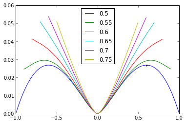
Let's graph the RMS capacitor current, as a function of duty cycle. If you go through some more algebra, you'll find out it has its maximum value at D = ±0.6. While we're at it, let's plot the RMS capacitor ripple for common-mode duty cycles different from 0.5: (the results are the same whether we go above 0.5 or below 0.5)
D = np.arange(-1,1,0.005)
def calcIcdc_ramp_symbolic(Da,Db):
  D = Da-Db
  D0 = (Da+Db)/2
  return abs(D)**1.5/(4*sqrt(3)) * sqrt(12*(D0-0.5)**2 + (1-abs(D))**2)
D0range = [0.5,0.55,0.6,0.65,0.7,0.75]
for D0 in D0range:
  Dlim = 1.0*D
  Dlim[abs(Dlim)+2*D0 > 2] = np.nan
  plt.plot(Dlim,calcIcdc_ramp_symbolic(D0 + Dlim/2, D0 - Dlim/2))
plt.plot(0.6,calcIcdc_ramp_symbolic(0.8,0.2),'.')
plt.legend(D0range,'upper center')
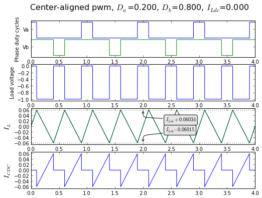
Let's just spot-check this for a few values to make sure we haven't made any obvious mistakes:
fig = plt.figure(figsize=(8, 6), dpi=80)
showpwmripple2(fig, t, 0.2, 0.8, I_Ldc=0, centeralign=True);
def calcIcdc_ramp_empirical(Da,Db):
  t = np.arange(0,4,0.0002)
  pwma = pwm(t,Da,centeralign=True)
  pwmb = pwm(t,Db,centeralign=True)
  Iab = calcripple(t,(pwma-pwmb))
  Icdc = calc_capacitor_ripple(pwma,pwmb,Iab,I_S=0)
  return rms(t,Icdc)

def checkIcdc_ramp(Da,Db):
  print 'Icdc rms ripple, empirical(%f,%f)=%f' % (
      Da,Db,calcIcdc_ramp_empirical(Da,Db))
  print 'Icdc rms ripple, symbolic(%f,%f)=%f' % (
      Da,Db,calcIcdc_ramp_symbolic(Da,Db))

checkIcdc_ramp(0.2,0.8)
checkIcdc_ramp(0.1,0.9)
checkIcdc_ramp(0.7,0.1)
Icdc rms ripple, empirical(0.200000,0.800000)=0.026831
Icdc rms ripple, symbolic(0.200000,0.800000)=0.026833
Icdc rms ripple, empirical(0.100000,0.900000)=0.020652
Icdc rms ripple, symbolic(0.100000,0.900000)=0.020656
Icdc rms ripple, empirical(0.700000,0.100000)=0.035497
Icdc rms ripple, symbolic(0.700000,0.100000)=0.035496
Pulse capacitor current
Pulse capacitor current is much simpler. It is equal to \( I_{Ldc} (1-|D|) \mathrm{sign}(D) \) in the intervals \( [t_1,t_2] \) and \( [t_4,t_5] \) (when voltage is applied across the load), a total time of \( |D|T \), and is equal to \( -DI_{Ldc} \) during the rest of the time when the load is short circuited, a total time of \( (1-|D|)T \).
def show_pulse_capacitor_current(fig, t, Da, Db, I_Ldc, centeralign=False):
    pwmA = pwm(t,Da,centeralign)
    pwmB = pwm(t,Db,centeralign)
    I_S = (Da-Db)*I_Ldc
    Icdc_pulse = I_Ldc*(pwmA-pwmB) - I_S
    ax=fig.add_subplot(1,1,1)
    ax.plot(t,Icdc_pulse)
    ax.set_ylim(createLimits(0.1,Icdc_pulse))
    return ax
fig = plt.figure()
show_pulse_capacitor_current(fig,t,0.7,0.1,I_Ldc=1.0,centeralign=True)
The RMS value of this waveform is easy to calculate, since it's piecewise constant: we just take the square root of the sums of squares of each constant, weighted by the total fraction of the time period it is active:
$$\begin{eqnarray} RMS(I _ {CDC\_pulse}) & = & \sqrt{|D| \times { I _ {CDC}}^2 \big| _ \text{Vdc across load} + (1-|D|) \times {I _ {CDC}}^2 \big| _ \text{shorted load} }\cr & = & I _ {Ldc}\sqrt{|D|(1-|D|)^2 + (1-|D|)D^2} \cr & = & I _ {Ldc}\sqrt{|D|(1 -|D|)}\sqrt{(1 -|D|) + |D|} \cr & = & I _ {Ldc}\sqrt{|D|(1 -|D|)} \end{eqnarray}$$
Total RMS capacitor current
We figured out that \( RMS(I _ {CDC\_ramp}) = \sqrt{|D|} \times RMS(I _ {L\_ripple}) \)
Now if we combine RMS values for ramp and pulse currents together, we get:
$$\begin{eqnarray} RMS(I _ {CDC}) & = & \sqrt{RMS(I _ {CDC\_ramp})^2 + RMS(I _ {CDC\_pulse})^2} \cr & = & \sqrt{ |D| \times RMS(I _ {L\_ripple})^2 + I _ {Ldc}^2 |D|(1-|D|)} \cr & = & \sqrt{ |D| } \sqrt{RMS(I _ {L\_ripple})^2 + (1-|D|)I _ {Ldc}^2} \end{eqnarray}$$
With \( D_0 = 0.5 \), this simplifies to
$$\begin{eqnarray} RMS(I _ {CDC}) & = & \sqrt{ |D| \times \frac{{I_R}^2}{48} + I _ {Ldc}^2 |D|(1-|D|)} \cr & = & \sqrt{ |D| (1-|D|) } \sqrt {\tfrac{27}{4}D^2(1-|D|)\left(\frac{I _ {R0}}{18}\right)^2 + I _ {Ldc}^2 } \end{eqnarray}$$
Blah, blah, blah, algebra, magic numbers, blah blah. So what? Here's what the function \( \frac{27}{4}D^2(1-|D|) \) looks like:
D = np.linspace(-1,1,100)
plt.plot(D,27*D*D*(1-abs(D))/4,2.0/3,1,'.')
plt.ylim(0,1.005);
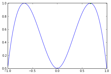
It has its maximum value of 1 at \( D=\pm \frac{2}{3} \).
This means that in order for ramp current and pulse current to have equal contributions to RMS capacitor ripple, even at \( D=\pm \frac{2}{3} \), \( I_{Ldc} \) would have to be 18 times smaller than \( I_{R0} \).
Here's what this case looks like:
fig = plt.figure(figsize=(8, 6), dpi=80)
split_Icdc_2(fig, t, 5.0/6, 1.0/6, I_Ldc=1.0/18, centeralign=True)
This is so near to \( I_{Ldc} = 0 \), that in normal cases, when \( I_{Ldc} \) is much larger, the net impact of inductor ripple current to the RMS capacitor current is essentially negligible. We'll talk more about this and other practical issues a bit later.
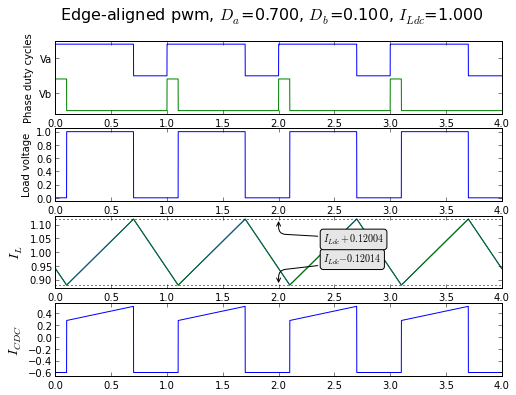
Edge-aligned PWM
So far, so good. But let's just cover the edge-aligned PWM case as well, just to be thorough.
fig = plt.figure(figsize=(8,6), dpi=80)
showpwmripple2(fig, t, 0.7, 0.1, I_Ldc=1.0, centeralign=False)
Again, we can do the same partitioning for analysis of peak and RMS currents. Fortunately the edge-aligned PWM case is easier to analyze.
Peak capacitor current, edge-aligned PWM
fig = plt.figure(figsize=(8, 6), dpi=80)
split_Icdc_1(fig, t, 0.7, 0.1, I_Ldc=1.0, centeralign=False)
The peak-to-peak capacitor current is the maximum load inductor current, which is \( \mathrm{peak}(I_{L}) = |I_{Ldc}| + \tfrac{1}{2}I_R = |I_{Ldc}| + \tfrac{1}{2}|D|(1-|D|)I_{R0} \).
The zero-to-peak values of capacitor current for positive power flow \( DI_{Ldc} > 0 \) are
$$\begin{eqnarray} \mathrm{peak_+} (I_ {CDC}) & = & |I_{Ldc}|(1-|D|) + \tfrac{1}{2}I_R \cr \mathrm{peak_-} (I_ {CDC}) & = & -DI_{Ldc} \end{eqnarray}$$
and for regenerative (negative) power flow \( DI_{Ldc} < 0 \) are
$$\begin{eqnarray} \mathrm{peak_+} (I_ {CDC}) & = & -DI_{Ldc} \cr \mathrm{peak_-} (I_ {CDC}) & = & -|I_{Ldc}|(1-|D|) - \tfrac{1}{2}I_R \end{eqnarray}$$
RMS capacitor current, edge-aligned PWM
Again, let's split up capacitor current the other way:
fig = plt.figure(figsize=(8, 6), dpi=80)
split_Icdc_2(fig, t, 0.7, 0.1, I_Ldc=1.0, centeralign=False)
Here's the contribution of ramp current, which is nonzero only for a time DT where it ramps from \( -I_R/2 \) to \( I_R/2 \):
D,T,Ir = sympy.symbols('D T I_R')
def f3(y0,y1,h):
    return h*(y0*y0 + y0*y1 + y1*y1)/3
integral_squared_ripple = f3(-Ir/2,Ir/2,abs(D)*T)
mean_squared_ripple = integral_squared_ripple/T
mean_squared_ripple
Take the square root of this and we just get
$$RMS(I _ {CDC\_ramp}) = \frac{I_R}{2\sqrt{3}}\sqrt{|D|} = \sqrt{|D|} \times RMS(I _ {L\_ripple})$$
and again, if we've already calculated the load inductor RMS ripple current, all we have to do to get the RMS of capacitor ramp current is multiply by this factor of \( \sqrt{|D|} \).
For pulse current, the RMS value is the same as in the center-aligned PWM case (same amplitude, half the frequency of center-aligned PWM):
$$RMS(I _ {CDC\_pulse}) = I _ {Ldc}\sqrt{|D|(1 -|D|)} $$
The total RMS current, just as in the center-aligned PWM case, is
$$RMS(I _ {CDC}) = \sqrt{|D|}\sqrt{I _ {L\_ripple}^2 + (1-|D|)I _ {Ldc}^2}$$
When we simplify it in terms of \( I_{R0} \) we get a slightly different answer, since the edge-aligned case produces twice the ripple current as center-aligned PWM:
$$\begin{eqnarray} RMS(I _ {CDC}) & = & \sqrt{ |D| \times \frac{{I_R}^2}{12} + I _ {Ldc}^2 |D|(1-|D|)} \cr & = & \sqrt{ |D| (1-|D|) } \sqrt {\tfrac{27}{4}D^2(1-|D|)\left(\frac{I _ {R0}}{9}\right)^2 + I _ {Ldc}^2 } \end{eqnarray}$$
but the end conclusion is still about the same: maximum contribution of ramp current to RMS, compared to pulse current, is at \( D = \pm \frac{2}{3} \), and even at that point the DC current has to be pretty small for the ramp current to contribute equally.
Harmonic amplitudes
Capacitor ramp current
For both the edge-aligned PWM case, and the center-aligned PWM case with common-mode duty cycle \( D_0 = \frac{1}{2} \), the capacitor ramp current waveform is zero except for a linear segment from \( -I_{pk} \) to \( I_{pk} \), with slope = \( (1-|D|)I _ {R0} \). For the edge aligned case, this occurs once per period for a time DT. For the center-aligned case, it occurs twice per PWM period for a time |D|T/2. The wave shape is the same for both, but at twice the frequency for center-aligned PWM, and the peak current \( I_{pk} \) is half as much.
(Here I'm going to be a little bit sloppy, and shift the waveform in time so that the ramp in the waveform is centered at t=0.)
We'll evaluate the Fourier coefficients for the edge-aligned case; the center-aligned case includes an additional factor of \( \frac{1}{2} \). Since there is only one linear segment of the waveform, we have only one integral to evaluate:
$$A_k = \frac{2}{T}\int _ {-T/2}^{T/2}{e^{2\pi jkt/T}}I _ {CDC\_ramp}(t)dt = \frac{2}{T}\int _ {-|D|T/2}^{|D|T/2}{e^{j2\pi kt/T}}(1-|D|)I _ {R0}\frac{t}{T} dt$$
Let's use sympy to help get those Fourier coefficients.
def calcRampCoeff(k,T=1):
  D,t,IR0 = sympy.symbols('D t I_{R0}')
  # for some reason sympy doesn't seem to handle complex
  # numbers very well in integration, so we'll help it along
  integrand_re = sympy.cos(2 * k * sympy.pi * t / T) * (1-abs(D))*IR0*t/T
  integrand_im = sympy.sin(2 * k * sympy.pi * t / T)* (1-abs(D))*IR0*t/T
  return sympy.simplify(2/T *
              (sympy.integrate(integrand_re,(t,-abs(D)*T/2,abs(D)*T/2))
           +1j*sympy.integrate(integrand_im,(t,-abs(D)*T/2,abs(D)*T/2))))
for k in range(1,6):
    display('A_%d = ' % k, calcRampCoeff(k))
A_1 =
A_2 =
A_3 =
A_4 =
A_5 =
It appears as though the general term is $$A_k = \frac{j(1-|D|)I _ {R0}(\sin k\pi |D| - k\pi |D| \cos k\pi |D|)}{k^2\pi ^2}$$ but let's double-check this just to be sure:
def Icdc_ramp_approx(D,kmax):
    def f(t):
        y = 0
        for k in range(1,kmax+1):
            kpiD = k*np.pi*abs(D)
            a_k = (sin(kpiD) - kpiD*cos(kpiD))
            A_k = a_k * (1-abs(D)) /k/k/np.pi/np.pi
            y += A_k*sin(2*np.pi*k*t)
        return y
    return f

def Icdc_ramp(D):
    def f(t):
        u = (t+0.5) % 1 - 0.5
        return u*(1-abs(D))*(abs(u)<abs(D)/2)
    return f

f = Icdc_ramp(0.6)
f_approx = Icdc_ramp_approx(0.6,10)
t = np.arange(-1,1,0.001)
plt.plot(t,f(t),t,f_approx(t))
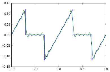
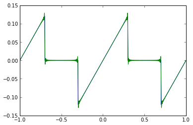
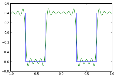
Not bad, although because of the step discontinuities there are Gibbs phenomena, so let's look at 100 Fourier coefficients:
f = Icdc_ramp(0.6)
f_approx = Icdc_ramp_approx(0.6,100)
t = np.arange(-1,1,0.001)
plt.plot(t,f(t),t,f_approx(t))
The harmonic content of the center-aligned case with \( D_0 \neq \frac{1}{2} \) is possible to calculate as well, but I'll leave that as an exercise for the interested reader.
Harmonic content of capacitor pulse current
Here the waveform is pretty simple just a two-level piecewise constant waveform.
fig = plt.figure()
show_pulse_capacitor_current(fig,t,0.8,0.2,I_Ldc=1.0,centeralign=False)

Except for its DC value, the harmonic amplitude of this is the same as any other waveform shifted up by a constant, so let's consider a square wave shifted so that its level near t=0 is at 0 and its level near t=± 0.5 is at \( sI_{Ldc} \) where \( s=\mathrm{sign}(D) \).
$$A_k = \frac{2}{T}\int_{-T/2}^{T/2}{e^{-2\pi jkt/T}}sI_{Ldc}dt $$
This looks like it's going to be pretty simple (smells like a sine function to me), and we could do it by hand, but let's give sympy a try:
def calcPulseCoeff(k,T=1):
  D,t,s,I_Ldc = sympy.symbols('D t s I_{Ldc}')
  # for some reason sympy doesn't seem to handle complex
  # numbers very well in integration, so we'll help it along
  integrand_re = sympy.cos(2 * k * sympy.pi * t / T) * s*I_Ldc
  integrand_im = sympy.sin(2 * k * sympy.pi * t / T)* s*I_Ldc
  return sympy.simplify(2/T *
              (sympy.integrate(integrand_re,(t,-abs(D)*T/2,abs(D)*T/2))
           +1j*sympy.integrate(integrand_im,(t,-abs(D)*T/2,abs(D)*T/2))))
for k in range(1,6):
    display('A_%d = ' % k, calcPulseCoeff(k))
A_1 =
A_2 =
A_3 =
A_4 =
A_5 =
Excellent! It's just $$A_k = \frac{2sI_{Ldc} \sin k\pi|D|}{k\pi} = \frac{2I_{Ldc} \sin k\pi D}{k\pi} $$
Let's verify:
def Icdc_pulse_approx(D,I_Ldc,kmax):
    def f(t):
        y = 0
        for k in range(1,kmax+1):
            A_k = 2*I_Ldc*sin(k*np.pi*D)/k/np.pi
            y += A_k*cos(2*np.pi*k*t)
        return y
    return f

def Icdc_pulse(D,I_Ldc):
    def f(t):
        u = (t+0.5) % 1 - 0.5
        return (abs(u)<abs(D)/2)*I_Ldc*np.sign(D) - D*I_Ldc
    return f

f = Icdc_pulse(0.6,1.0)
f_approx = Icdc_pulse_approx(0.6,1.0,10)
t = np.arange(-1,1,0.001)
plt.plot(t,f(t),t,f_approx(t))

plt.figure()
f = Icdc_pulse(-0.6,1.0)
f_approx = Icdc_pulse_approx(-0.6,1.0,10)
t = np.arange(-1,1,0.001)
plt.plot(t,f(t),t,f_approx(t))
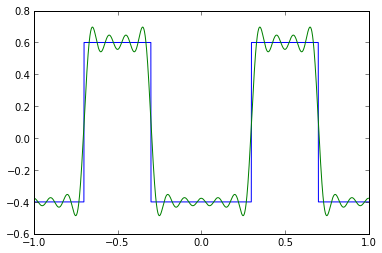
There's those Gibbs ears again!
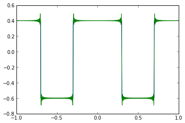
f = Icdc_pulse(0.6,1.0)
f_approx = Icdc_pulse_approx(0.6,1.0,100)
t = np.arange(-1,1,0.001)
plt.plot(t,f(t),t,f_approx(t))
So the total harmonic amplitude, including both ramp and pulse components of capacitor current, is
$$A _ k = \underbrace{\frac{j(1-|D|)(\sin k\pi |D| - k\pi |D| \cos k\pi |D|)}{k^2\pi ^2}} _ {\text{ramp current}} + \underbrace{\frac{2I _ {Ldc} \sin k\pi D}{k\pi}} _ {\text{pulse current}}$$
3-phase PWM
Yet another exercise for the reader. Or you'll see it sometime in an appnote at http://www.microchip.com/motorcontrol when I get a chance to write one.
Now what?
Oh, my head aches with algebra! Thank you for your patience if you've read this far. It's time to summarize these results.
Summary
Here's a summary of capacitor ripple current statistics for H-bridge PWM.
Remember our definitions:
\( D = D_a - D_b \) is the effective load duty cycle
\( D_0 = (D_a + D_b)/2 \) is the common-mode duty cycle
\( I_{CDC} \) is the current flowing out of the DC link capacitor
\( I_S = DI_{Ldc} \) is the supply current
\( I_{R0} = V_{DC}T/L \) is a reference current that simplifies calculation of these statistics.
\( I_R = |D|(1-|D|)I_{R0} \) is a differential duty-cycle dependent ripple current
\( I_{R2} = 2|D||D_0-\tfrac{1}{2}|I_{R0} \) is a common-mode duty-cycle dependent ripple current
\( I_{Lpk} \) = Mean-to-peak load current ripple
\( I_{Lrms} \) = RMS load current ripple (does not include DC)
Here are statistics about \( I_{CDC} \):
Information from Part 1:
| PWM type | \( I_{Lpk} \) | \( I_{Lrms} \) | fundamental frequency |
|---|---|---|---|
| edge-aligned | \( \tfrac{1}{2}I_R \) | \( \frac{1}{2\sqrt{3}}I_R \) | \( f_{PWM} = 1/T \) |
| center-aligned (common-mode = 0.5) |
\( \tfrac{1}{4}I_R \) | \( \frac{1}{4\sqrt{3}}I_R \) | \( 2f_{PWM} \) |
| center-aligned (common-mode ≠ 0.5) |
\( \tfrac{I_R+I_{R2}}{4} \) | \( \frac{|D|\sqrt{12(D_0-\tfrac{1}{2})^2 + (1-|D|)^2}}{4\sqrt{3}}I_{R0} \) | \( {f_{PWM}}^ * \) |
*1st harmonic of capacitor current in center-aligned PWM has low amplitude if D0 is close to 0.5
These statistics about DC link capacitor current can be expressed independent of the PWM type:
| statistic | symbol | value | conditions |
|---|---|---|---|
| peak-to-peak | \( I_{CDCpkpk} \) | \( |I_{Ldc}| + I_{Lpk} \) | |
| positive peak | \( I_{CDCpeak+} \) | \( |I_{Ldc}|(1-|D|) + I_{Lpk} \) | \( I_S > 0 \) (positive power) |
| negative peak | \( I_{CDCpeak-} \) | \( -I_S \) | |
| positive peak | \( I_{CDCpeak+} \) | \( -I_S \) | \( I_S < 0 \) (regeneration) |
| negative peak | \( I_{CDCpeak-} \) | \( -|I_{Ldc}|(1-|D|) - I_{Lpk} \) | |
| RMS | \( I_{CDCrms} \) | \( \sqrt{|D|}\sqrt{{I_{Lrms}}^2 + (1-|D|)I_{Ldc}^2} \) | |
| amplitude of kth harmonic |
\( A_k \) | $$\underbrace{\frac{j(1-|D|) I _ {R0}(\sin k\pi |D| - k\pi |D| \cos k\pi |D|)}{mk^2\pi ^2}} _ {\text{ramp current}} + \underbrace{\frac{2I _ {Ldc} \sin k\pi D}{k\pi}} _ {\text{pulse current}}$$ | * |
* \( m=1 \) for edge-aligned PWM, \( m=2 \) for center-aligned PWM with \( D_0 = \tfrac{1}{2} \). Calculating \( A_k \) for the general case of center-aligned PWM (\( D_0 \neq \tfrac{1}{2} \)) is an exercise for the reader.
Now that we have all these gory equations, next time we'll talk about some of the practical issues related to capacitor and inductor ripple current.
Happy switching!
© 2013 Jason M. Sachs, all rights reserved.
Stay tuned for a link to this code in an IPython Notebook. I'll put it up on the web, and I do plan to release this in an open-source license, I just have to do a little more homework before I pick the right one.


- Comments
- Write a Comment Select to add a comment
To post reply to a comment, click on the 'reply' button attached to each comment. To post a new comment (not a reply to a comment) check out the 'Write a Comment' tab at the top of the comments.
Please login (on the right) if you already have an account on this platform.
Otherwise, please use this form to register (free) an join one of the largest online community for Electrical/Embedded/DSP/FPGA/ML engineers: