How to Estimate Encoder Velocity Without Making Stupid Mistakes: Part II (Tracking Loops and PLLs)

Information Theory and Estimation
(well, some handwaving at least)

If you get into hard-core estimation theory, you'll deal with all sorts of matrix equations to deal with multiple variables and the cross-correlation of their probability distributions. There's terms like covariance matrices and Gram-Schmidt Orthogonalization and the Fisher Information Matrix and the Cramer-Rao Bound. I once understood these really well for a few weeks while taking a class in college. Alas, that light bulb has dimmed for me....

Anyway, don't worry about trying to understand this stuff. One major take-away from it is that the concepts of standard deviation (how much variation there is in a measurement due to randomness) and information are related. The Cramer-Rao bound basically says that information and variance (the square of standard deviation) are inversely related: the more variance your measurements have, the less information you have.

For Gaussian distributions, the relationships are exact, and if I combine unbiased measurements of the same underlying parameter M in an optimal manner, the amount of information accumulates linearly. So if I have a measurement M₁ of that parameter with a variance of 3.0 (information = 1/3), and an independent, uncorrelated measurement M₂ of the same parameter with a variance of 6.0 (information = 1/6), then the optimal combination of the two will yield a combined measurement \( \hat{M} \) with a variance of 2.0 (information = 1/2 = 1/3 + 1/6). It turns out that this optimal combination happens to be \( \hat{M} = \frac{2}{3}M_1 + \frac{1}{3}M_2 \). This is a weighted linear sum of the individual measurements: the weights always sum to 1.0, and the weights have the same proportion as each measurement's amount of information.

So one central concept of estimation is that you try to make optimal use of the information you have. If I combine measurements in another way, I will have less information. (With the M example before, if I make the naive estimate \( \hat{M} = \frac{1}{2}M_1 + \frac{1}{2}M_2 \), then the resulting variance happens to be \( (\frac{1}{2})^2 \times 3.0 + (\frac{1}{2})^2 \times 6.0 = 2.25 \), which is larger, so my estimate is slightly less likely to be as accurate.)

Back to our pendulum + encoder example, what do we know, and what kind of errors do we have?

We know the basic equations of the pendulum's motion; most significantly, knowing the pendulum position at one instant in time means that we are fairly likely to know it at a time shortly thereafter. The position measurements are highly correlated, so we should try to make the best use of all measurements we can take. Same thing with the velocity: as long as the torque on the pendulum isn't too high, knowing the pendulum velocity at one instant means we are fairly likely to know it at a time shortly thereafter.

Here's what errors prevent us from knowing the pendulum position with perfect precision:

• The position measurements have quantization errors, some due to the fact that we are using an encoder with finite resolution, and some due to the fact that the encoder edges may contain small position errors due to manufacturing tolerances. (I discussed this in a previous article.)
• The position measurements have noise: since it's a digital system this is minimal, but we can occasionally get encoder glitch pulses.
• If we stop paying attention to the pendulum for a few seconds, and someone spins it around a few times when we're not looking, we cannot tell the difference: we have no absolute reference for the number of physical rotations made by the pendulum.
• We may not know all of the pendulum parameters exactly (gravity, pendulum length, mass, viscous drag)
• We may not be able to model some of the dynamics exactly (permanent magnets)
• We may not be able to predict the disturbances exactly (the electromagnetic pulses, or someone coming by and giving it a whack)

The best estimators are the ones that take all these effects into account, reduce the net estimation error, and are robust to unexpected mistakes. The idea of robustness is subtle: if you design an estimator that's great when you know the pendulum parameters exactly and only takes one encoder reading per second, it could still give you a very low error, but then someone squirts WD-40 into the pendulum pivot to change the viscous drag and the estimator starts being way off.

What's wrong with the types of estimators we mentioned in Part I? Well, nothing really; they're simple, but they're just not optimal, or even close. If you're taking position measurements 10,000 times a second, and you compute velocity by taking each position measurement and subtracting off the position measured 1 second earlier, then you ignore all the potential information available in those other 9,998 readings between the two.

Common Structures of More Sophisticated Estimators

With that, let's go quickly over a small menagerie of estimator structures.

• Phase-locked loops (PLLs) — given oscillating inputs, a variable-frequency oscillator attempts to follow those inputs by using a phase detector and a feedback loop to try to drive the phase error to zero.
• Tracking loops — an estimator attempts to follow the input by using an error and a feedback loop to try to drive the error to zero. (Similar to a PLL, but without the oscillating part.)
• Luenberger observers — a type of tracking loop that tries to simulate the dynamics of the real system, and adds a corrective term based on a fixed gain applied to the difference between real and simulated systems.
• Adaptive filters (e.g. Least Mean Square or Recursive Least Squares filters) — a type of tracking loop that tries to simulate the dynamics of the real system, then uses the error between real and simulated system to adjust the parameters of the simulation
• Kalman filters — essentially a Luenberger observer with a variable gain, where the variable gain is derived from estimates of measurement noise to determine the optimal gain.

Adaptive and Kalman filters are best used in cases where the sources of noise or error are "ordinary" — that is, they have a distribution that is somewhat Gaussian in character and uncorrelated with the measurements. Kalman filters were developed for guidance systems in the aerospace industry: things like radar and GPS and trajectory tracking are really good applications. Kalman filters also do very well when the signal-to-noise ratio varies with time, as they can adapt to such a situation. I often read articles that try to apply Kalman filters in sensorless position estimators used in motor control, and it's saddening to see this, since in these applications the errors are more often due to imperfect cancellation of coupling between system states, instead of random noise, and the errors are anything but Gaussian or uncorrelated. Likewise in this encoder application: quantization noise from a position encoder is not really a good match for an adaptive filter or Kalman filter, so I won't discuss it further.

The remaining three structures mentioned here are similar. I'll cover PLLs and tracking loops next, leaving Luenberger observers for Part III. Since tracking loops are fairly general, and PLLs and Luenberger observers are specific types of tracking loops, it makes sense to cover tracking loops first.

Tracking loops

Here's a really simple example. Let's say we have a continuous position signal, and when we measure it, we get the position signal along with additive Gaussian white noise:

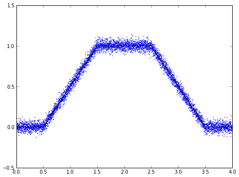
Now, your first reaction might be, "Hey, let's just filter out the noise with a low-pass filter!" That's not such a bad idea, so let's do it:

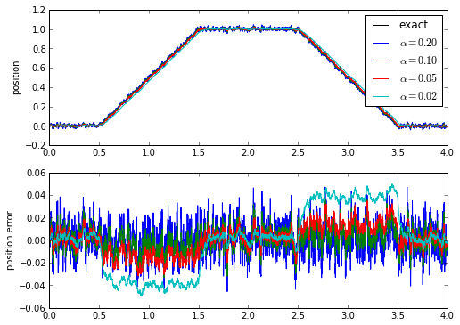
And here we have the same problem we ran into when we were looking at evaluating algorithms in Part 1.5: there's a tradeoff between noise level and the effects of phase lag and time delay. A simple low-pass filter doesn't do very well tracking ramp waveforms: the time delay causes a DC offset.

With a tracking loop, we try to model the system and drive the steady-state error to zero. Let's model our system as a velocity that varies, and integrate the estimated velocity to get position. The velocity will be the output of a proportional-integral control loop driven by the position error.

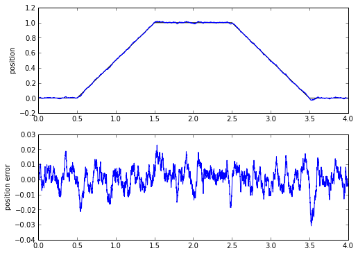
The RMS and peak error here are less than in the 1-pole low-pass filter. Not only that, but in the process, we get an estimate of velocity! We actually get two estimates of velocity. One is the integrator of the PI loop used in the tracking loop, the other is the output of the PI loop. Let's plot these (integrator in blue, PI output in yellow):

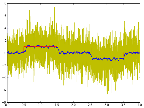
The PI output looks horrible; the PI integrator looks okay. (There's quite a bit of noise here, so it's really difficult to get a good output signal.)

Which one is better to use? Well, for display purposes, I'd use the integrator value; it doesn't contain high frequency noise. For input into a feedback loop (like a velocity controller), I might use the PI output directly, since the high-frequency stuff will most likely get filtered out anyway.

So the tracking loop is better than a plain low-pass filter, right?

Well, in reality there's a trick here. This tracking loop is a linear filter, so it can be written as a regular IIR low-pass filter. The thing is, it's a 2nd-order filter, whereas we compared it against a 1st-order low-pass filter, so that's not really fair.

But by writing it as a tracking loop, we get a more physical meaning to filter state variables — and more importantly, if we want to, we can deal with nonlinear system behavior using a tracking loop that includes nonlinear elements.

For those of you interested in the Laplace-domain algebra (for the rest of you, skip to the next section) the estimated position \( \hat{x} \) and estimated velocity \( \hat{v} \) behave like this (quick refresher: \( 1/s \) is the Laplace-domain equivalent of an integrator):

$$\begin{eqnarray} \hat{x}&=&\frac{1}{s}\hat{v}\cr \hat{v}&=&(\frac{k_i}{s} + k_p)(x-\hat{x}) \end{eqnarray}$$

which we can then solve to get

$$\hat{x} = \frac{k_ps + k_i}{s^2}(x-\hat{x}) $$

and then (after a little more algebraic manipulation)

$$\hat{x} = \frac{\frac{k_p}{k_i}s + 1}{\frac{1}{k_i}s^2 + \frac{k_p}{k_i}s + 1}x $$

which is just a low-pass filter with two poles and one zero, whereas the 1-pole low-pass filter is

$$\hat{x} = \frac{1}{\tau s+1}x$$

The error in these systems is

$$\tilde{x} = x-\hat{x} = \frac{\frac{1}{k_i}s^2}{\frac{1}{k_i}s^2 + \frac{k_p}{k_i}s + 1}x $$

and

$$\tilde{x} = \frac{\tau s}{\tau s+1}x$$

If we use the Final Value Theorem, the steady-state error for both of these to a position step input is zero, but the steady-state error for a position ramp input (velocity step input) is nonzero for the 1-pole low-pass filter, whereas it is still zero for the tracking loop. This is because of the zero in the tracking loop's transfer function.

Need to track position in case of constant acceleration? Then go ahead and add another integrator... just make sure you analyze the transfer function and add a proportional term to that integrator so the resulting filter is stable.

Phase-locked loops (PLL)

Tracking loops are great! There is a special class of tracking loops to handle problems where it is important to lock onto the phase or frequency of a periodic signal. These are called phase-locked loops (go figure!), and they usually consist of the following structure:

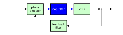
The idea is that you have a voltage-controlled oscillator (VCO) creating some output, that goes through a feedback filter, gets compared in phase against the input with a phase detector, and the phase error signal goes through a loop filter before it is used as a control signal for the VCO. The loop filter's input and output are essentially DC signals proportional to output frequency; the other signals in the diagram are periodic signals. The feedback filter is usually just a passthrough (no filter) or a frequency divider. Most microcontrollers these days with PLL-based clocks have a divide-by-N block in the feedback filter, which has the net effect that the output of the PLL multiplies the input frequency by N. This way you can take, for example, an 8 MHz crystal oscillator and turn it into a 128MHz clock signal on the chip: as a result, you don't need to distribute high-frequency clock signals on your printed circuit board, just a low-frequency clock, and it will get multiplied up internal to the microcontroller. At steady-state, the signals in the PLL are sine waves or square waves, except for the VCO input which is a DC voltage; the inputs to the phase detector line up in phase. (Digital PLLs are possible as well, in which case the VCO is replaced by a digitally-controlled oscillator with a digital input representing the control frequency.)

One simple example of a PLL is where the phase detector is a multiplier that acts on sine waves, the loop filter is an integrator, and there is no feedback filter, just a passthrough. In this case you have

$$\begin{eqnarray} V_{in} &=& A \sin \phi_i(t) \cr \phi_i(t) &\approx& \omega t + \phi_{i0}\cr V_{out} &=& B \sin \phi_o(t) \cr V_{pd} &=& V_{in}V_{out} = AB \sin \phi_i(t) \sin \phi_o(t) \cr &=& \frac{AB}{2} (\cos (\phi_i(t) - \phi_o(t)) + \cos(\phi_i(t) + \phi_o(t)))
\end{eqnarray}$$

The phase detector outputs a sum and difference frequency: if the output frequency is the about same, then the sum term \( \cos(\phi_i(t) + \phi_o(t)) \) is about double the input frequency, and the difference term \( \cos(\phi_i(t) - \phi_o(t)) \) is at low frequency. The loop filter is designed to filter out the double-frequency term, and integrate the low-frequency term:

$$\begin{eqnarray} V_{VCO_in} &\approx& K\sin(\phi_i(t) - \phi_o(t)) + f_0 \end{eqnarray}$$

This will reach equilibrium with constant phase difference between \( \phi_i(t) \) and \( \phi_o(t) \) → the loop locks onto the input phase!

In general, phase-locked loops with sine-wave signals tend to have dynamics that look like this:

$$\begin{eqnarray} \frac{dx}{dt} &=& A\sin \tilde{\phi} = A\sin(\phi_i - \phi_o) \cr \tilde{\omega} &=& -x - B\sin \tilde{\phi} - C\sin 2\omega t\cr \frac{d\tilde{\phi}}{dt} &=& \tilde{\omega} \end{eqnarray}$$

If you're not familiar with these types of equations, your eyes may glaze over. It turns out that they have a very similar structure to the rigid pendulum equations above! (The plain pendulum equations, with only gravity, inertia, and damping — no magnets.) With a good loop filter, the high frequency amplitude C is very small, and we can neglect this term. At low values of phase error \( \tilde{\phi} \), the phase error oscillates with a characteristic frequency and a decaying amplitude. At high values of \( \tilde{\phi} \) there are some weird behaviors, that are similar to that of a pendulum spinning around before it settles down.

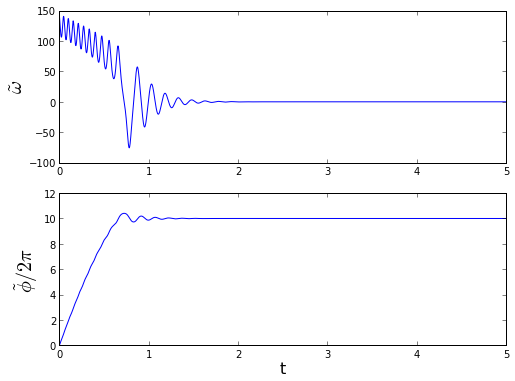
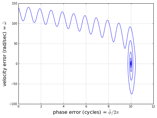
This is typical of the behavior of phase-locked loops: because there is no absolute phase reference, with a large initial frequency error, you can get cycle slips before the loop locks onto the input signal. It is often useful to plot the behavior of phase and frequency error in phase space, rather than as a pair of time-series plots:

We can also try graphing a bunch of trials with different initial conditions:

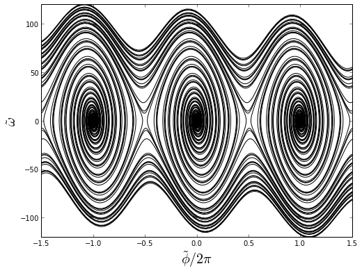
Crazy-looking, huh? The trajectory in phase space oscillates until it gets close enough to one of the stable points, and then swirls around with decreasing amplitude.

PLLs should always be tuned properly — there are tradeoffs in choosing the two gains A and B that affect loop bandwidth and damping, and also noise rejection and lock acquisition time. I may cover that in another article, but for now we'll try to keep things at a fairly high level.

Is a PLL relevant to our encoder example? Well, yes and no.

The "no" answer (PLLs are not relevant) is true if we use a dedicated encoder counter; aside from initial location via an index pulse, the encoder counter will always give us an exact position. We don't need to guess whether the encoder is at position X or position X+1 or position X+2. If we want to smooth out the position and estimate velocity, we can use a regular tracking loop and know with certainty that we will always end up at the right position.

The "yes" answer (PLLs are relevant) is true if we use an encoder counter in a very noisy system. We may get spurious encoder counts that cause us to slip in the 4-count encoder cycle. (00 -> 01 -> 11 -> 10 -> 00) In this case a PLL can be very useful because it will reject high frequency glitches. Alternatively, if we are using position sensors that are more analog in nature (resolvers or analog hall sensors, or sensorless estimators), PLLs are very appropriate, especially if they are a set of analog sensors. Here's why:

Scalar vs. vector PLLs

Let's look at that good old sine wave again:

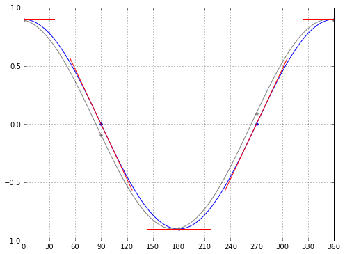
Here's two sine waves, actually; the two are 6° apart in phase. (Six degrees of separation! Ha! Sorry, couldn't resist.) Look at the difference between the resulting signals at different points in the cycle. Near 90° and 270°, when the signal is near zero, the slope is large, and we can easily distinguish these two signals by their values at the same time. When the signal is near its extremes, however, the slope is near zero, and the signals are very close to each other. Higher slope gives us more phase information. We also can't tell exactly where the signal is in phase just by looking at it at one point in time: if the signal value is 0, is the phase at 90° or 270°? They have the same value. Or if these signals are representing the cosine of position, we can't tell whether the position is moving backwards or forwards, since \( cos(x) = cos(-x) \).

Now suppose we have two sine waves 90° apart:

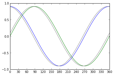
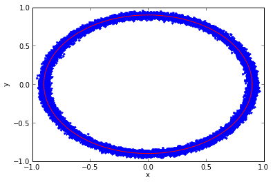
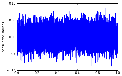
Here we can estimate phase by using both signals! When one signal is at its extreme, and the slope is zero, we get very little information, but we can get useful information from the other signal, which is passing through zero and is at maximum slope. It turns out that the optimum way to estimate phase angle from given measurements of these two signals at a single instant is to use the arctangent: φ = atan2(y,x). We can identify the phase angle of these signals at any point in the cycle, and can distinguish whether the phase is going forwards and backwards. We can even estimate the error of the phase estimate: if the signals have amplitude A, and there is additive Gaussian white noise on both signals with rms value n, where n is small compared to A, it turns out that the resulting error in the phase estimate has rms value of n/A in radians, independent of phase:

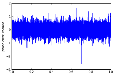
Now suppose we have a high noise situation:

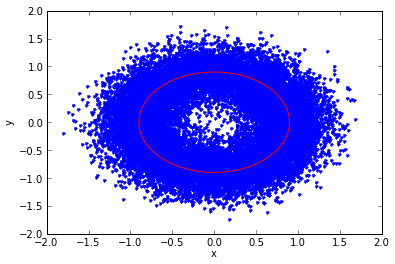
Oh, dear. When the signal plus noise results in readings near (0,0) it gets kind of nasty, and the phase can suddenly flip around. Let's say we're making measurements of x and y every so often, then calculating the phase using the arctangent, and we derive successive angle estimates of 3°, 68°, -152°, -20°, 17°, 63°. Did the angle wander near zero, with a noise spike at 68° and -152°, which we should filter out? Or did it increase moderately fast, wrapping around 1 full cycle from 3°, 68°, 208°, 340°, 377°, 423°? We can't tell; the principal angles are the same.

One big problem with the atan2() method is that it only tells us the principal angle, with no regard to past history. If we want to construct a coherent history, we have to use an unwrapping function:

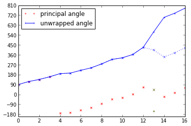
And the problem is that in signals with high frequency content, one single sample that has a noise spike can lead to a cycle slip, because we can't distinguish a noise spike from a legitimate change in value. In the graph above, two different angle values measured at index 13 cause us to pick different numbers of revolutions in unwrapped angle. Lowpass filtering after the arctan will not help us out; lowpass filtering before the arctan will cause a phase error. There are two better solutions:

• sampling faster (this lets us see large spikes more easily) and slew-rate limiting the unwrapped output
• a phase-locked loop

A phase-locked loop will filter out noise more easily. Since we have two signals x and y, we need a vector PLL rather than a scalar PLL. One of the best approaches for a vector PLL with two sine waves 90 degrees out of phase, is a quadrature mixer: if we use a phase detector (PD) that computes the cross product between estimated and measured vectors, we get a very nice result. If the incoming angle φ is unknown, then

$$\begin{eqnarray} x &=& A \cos \phi\cr y &=& A \sin \phi\cr \hat{x} &=& \cos \hat{\phi}\cr \hat{y} &=& \sin \hat{\phi}\cr \mathrm{PD\ output} &=& \hat{x}y - \hat{y}x \cr &=& A \cos \hat{\phi} \sin \phi - A \sin \hat{\phi} \cos \phi \cr &=& A \sin (\phi - \hat{\phi})\cr &=& A \sin \tilde{\phi} \end{eqnarray}$$

Just as a reminder: the ^ terms are estimates; the ~ terms are errors, and the "plain" x and y are measurements.

There's no high frequency term to filter out here! That's one of the big advantages of a vector PLL over a scalar PLL; if we can measure (or derive from a series of measurements) quadrature components that are proportional to \( \cos \phi \) and \( \sin \phi \), we don't need as much of a filter. In reality, imperfect phase and amplitude relationship means that there will be some double-frequency term that makes it into the output of the phase detector, but the amplitude should be fairly small.

A vector PLL is a tracking loop on the x and y measurements, but based on state variables in terms of phase angle and its derivatives. (Or to say it a different way: measurements are in rectangular coordinates, but state variables are in polar coordinates.) This is kind of the best of both worlds, because we can use information about reasonable changes in angle and amplitude, but not have to worry about angle unwrapping errors if we get single noise spikes, since we don't ever have to convert from principal angle (-180° to +180°) to unwrapped angle. If noise at one particular instant causes our (x,y) measurements to come close to zero, the phase detector output will be small and the effect on the PLL output will be minimal.

Okay, well what does this have to do with encoders?

You caught me — we've veered off onto a tangent, and it doesn't have much to do with digital encoders. (Resolvers and analog sensors, yes. Digital encoders, no.) But I wanted you to see the big picture before delving into the world of observers.

Summary

Tracking loops

• Useful for combining information from many samples to minimize the effect on noise
• Very general, with many specialized types (PLLs, Kalman Filters, observers, etc.)
• Usually with zero steady-state error even from ramp inputs
• Have filter state which has physical meaning
• Linear tracking loops are a type of low-pass filter, but general low pass filters do not have zero steady-state error from ramp inputs, and don't necessarily have filter state that has physical meaning

Phase-locked loops

• A tracking loop for periodic signals, where an absolute phase reference cannot be distinguished (e.g. 0° vs. 360° vs. 720°)
• Cycle slips are possible
• A divider in the feedback path can make the PLL act like a frequency multiplier
• Scalar PLLs have to filter out high-frequency components of phase detector output
• Phase estimation in vector systems is superior to phase estimation in scalar systems, where ambiguity in direction and phase cannot be prevented (analogous to the difference between the two types of arctangent: the two-input atan2() and the single-input atan() )
• Phase detection yields higher information when the slope of signal change is higher, and lower information when the incoming signal is at a minimum or maximum
• Phase detectors in vector PLLs can have a much smaller high-frequency component, and therefore require less filtering
• Vector PLLs that use quadrature mixers are superior to systems using arctan() + unwrap + tracking loop, because they are more immune to spurious cycle slips caused by noise spikes

Hope you learned something useful, and happy tracking!

Next up: Observers!

© 2013 Jason M. Sachs, all rights reserved.