First-Order Systems: The Happy Family
Все счастли́вые се́мьи похо́жи друг на дру́га, ка́ждая несчастли́вая семья́ несчастли́ва по-сво́ему.
— Лев Николаевич Толстой, Анна Каренина
Happy families are all alike; every unhappy family is unhappy in its own way.
— Lev Nicholaevich Tolstoy, Anna Karenina
I was going to write an article about second-order systems, but then realized that it would be premature to do so, without starting off on the subject of first-order systems.
Warning: this article isn't exciting. Sorry, it is what it is; that's the nature of first-order systems.

I'm sure you've run into first-order systems before. The RC filter is probably the most common one. It has a differential equation \( \frac{dV_{out}}{dt} = \frac{1}{RC}\left(V_{in}-V_{out}\right) \), and a transfer function of \( \frac{V_{out}}{V_{in}} = \frac{1}{RCs+1} \).
Time response
Here's what the unit step response of the RC filter looks like:
import numpy as np
import matplotlib.pyplot as plt

t = np.arange(-0.5,5.5,0.001)
plt.plot(t,t>0)
plt.plot(t,(t>0)*(1-np.exp(-t)))
plt.plot([0,1],[0,1],'-.')
plt.xlim([-0.5,5.5])
plt.ylim([-0.05,1.05])
plt.grid('on')
plt.xlabel(r'$t/\tau$',fontsize=16)
plt.suptitle('Unit step response of an RC filter with time constant $\\tau=RC$',
             fontsize=12)
plt.legend(['$V_{in}$','$V_{out}$'],'best',fontsize=16);
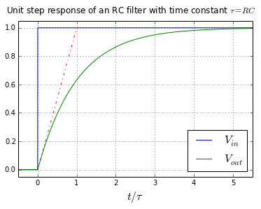
Some things to note:
- The final value of the step response is 1 (e.g. Vout = Vin)
- The initial value right after the step is 0, so the output waveform is continuous
- The step response is a decaying exponential with time constant τ = RC
- The slope of the output changes instantaneously after the step to a value of 1/τ
And there's not much else to say. All first order systems can be modeled in a general way as follows, for input u, output y, and internal state x:
$$ \begin{eqnarray} \frac{dx}{dt} &=& \frac{x-u}{\tau}\cr y &=& ax + bu \end{eqnarray}$$
This produces a system with transfer function \( H(s) = \frac{Y(s)}{U(s)} = b + \frac{a}{\tau s + 1} \), which has a time response after t=0 of \( b+a\left(1-e^{-t/\tau}\right) \) that looks like this:
def plot_firstorder(a=1,b=0,title=None):
    xlim = [-0.5,5.5]
    t = np.arange(xlim[0],xlim[1],0.001)
    plt.plot(t,(t>0)*(a+b-a*np.exp(-t)))
    plt.plot([0,1],[b,a+b],'-.')
    plt.plot(xlim,[a+b,a+b],'--g')
    plt.xlim(xlim)
    yticks = [(0,0)]
    if b != 0:
        yticks += [(b,'b')]
    if a+b != 0:
        yticks += [(a+b,'a+b')]
    yticks = sorted(yticks, key=(lambda x: x[0]))
    (yticks, yticklabels) = zip(*yticks)
    ymin = yticks[0]
    ymax = yticks[-1]
    plt.ylim([ymin-0.05*(ymax-ymin), ymax+0.05*(ymax-ymin)])
    plt.yticks(yticks,yticklabels)
    plt.xlabel(r'$t/\tau$',fontsize=16)
    title = ('Unit step response of a first-order system with time constant $\\tau$'
             if title is None else title)
    plt.suptitle(title, fontsize=12);

plot_firstorder(a=1,b=0.2)
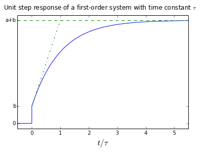
Again, some things to note:
- The final value of the step response is a+b
- The initial value right after the step is b
- The step response is a decaying exponential with time constant τ
- The slope of the output changes instantaneously after the step to a value of 1/τ
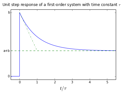
It's possible for either a or b to be negative, but that's about all that can change here.
plot_firstorder(a=-0.6,b=1)
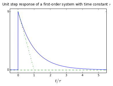
If a = -b, then we have a high-pass filter, which returns to a final value of zero:
plot_firstorder(a=-1,b=1)
Frequency response
If we create a Bode plot of the result, we'll see this:
# skip this Python code if you're not interested

def bodeplot_firstorder(a=1,b=0.0001):
    xlim = [-2,6]
    omega = np.logspace(xlim[0],xlim[1],300)
    lxlim = [omega[0],omega[-1]]
    Hfunc = lambda omega: b+a/(1j*omega+1)
    db = lambda x: 20*np.log(np.abs(x))
    ang = lambda x: np.angle(x,deg=True)
    H = Hfunc(omega)
    H0 = Hfunc(0)
    Hinf = Hfunc(1e9)
    fig = plt.figure(figsize=(8,6))
    ax = fig.add_subplot(2,1,1)
    ax.semilogx(omega,db(H))
    if a*b>=0 or abs(a) > 1.1*abs(b):
        asymptote = a/1j/omega
    else:
        asymptote = a*1j*omega
    ax.plot(omega,20*np.log(np.abs(asymptote)),'--g')
    ax.set_ylabel(r'$\log |H(\omega)|$', fontsize=16)
    ylim = [min(db(H)), max(db(H))]
    ax.set_ylim(1.05*ylim[0]-0.05*ylim[1],1.05*ylim[1]-0.05*ylim[0])
    yticks = [(db(Hinf), 'log a')]
    xticks = [(1,'1')]
    if abs(a) != abs(b):
        xticks += [(abs(a/b),'a/b')]
        yticks += [(db(H0), 'log b')]
    ax.set_yticks([tick[0] for tick in yticks])
    ax.set_yticklabels([tick[1] for tick in yticks])
    ax.set_xticks([tick[0] for tick in xticks])
    ax.set_xticklabels([tick[1] for tick in xticks])
    ax.grid('on')

    ax = fig.add_subplot(2,1,2)
    ax.semilogx(omega,ang(H))
    yt=np.arange(np.min(ang(H))//15*15,np.max(ang(H))+15,15)
    ax.plot([1,abs(a/b)],[ang(Hfunc(1)), ang(Hfunc(abs(a/b)))],'.')
    ax.set_yticks(yt)
    ax.set_ylabel(r'$\measuredangle H(\omega)$',fontsize=16)
    ax.set_xlabel(r'$\omega\tau$',fontsize=16)
    ax.set_xticks([tick[0] for tick in xticks])
    ax.set_xticklabels([tick[1] for tick in xticks])
    ax.grid('on')

bodeplot_firstorder(a=1,b=0.0001)
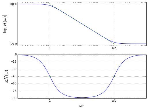
Things to note:
- The term \( \frac{a}{\tau s+1} \) contains a pole at \( \omega = \frac{1}{\tau} \)
- The constant term b forms a zero that, if present, counters the pole
- The magnitude of the transfer function decreases at 20dB/decade for frequencies ω > 1/τ, until it reaches a point where the constant term b is larger than the rest of the transfer function
- The phase of the transfer function goes from 0° to -90° because of the pole, but then returns to 0° because of the zero.
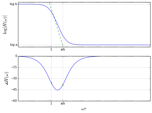
If one of the terms is negative, it does not affect the magnitude plot, but it does affect the phase:
bodeplot_firstorder(a=-1,b=0.0001)
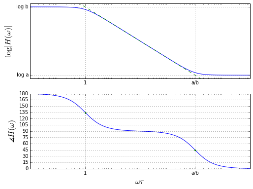
If b and a are not separated as much, the zero kicks in shortly after the pole:
bodeplot_firstorder(a=1,b=0.2)
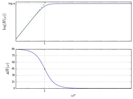
For a high-pass filter with a = -b, it changes the waveform somewhat:
bodeplot_firstorder(a=-1,b=1)
Following error of first-order systems
Back to the time domain....
The following error or tracking error of a first-order system measures how closely a particular first-order system is able to track its input. This really only makes sense for systems with unity gain and zero steady-state error, so we'll only consider first-order systems with b=0 and a=1, namely \( H(s) = \frac{1}{\tau s+1} \).
Step input
We've already seen how the first-order system tracks a step input:

There's an initial error, but it decays to zero steady-state error with time constant τ.
Ramp input
Here's what happens if you pass in a ramp input:
t = np.arange(-0.5,5.5,0.001)
tau = 1
Vin = (t>0)*t
Vout = (t>0)*(t-tau*(1-np.exp(-t/tau)))

def ploterror(t,Vin,Vout,title):
    fig = plt.figure(figsize=(8,6))
    ax = fig.add_subplot(2,1,1)
    ax.plot(t,Vin)
    ax.plot(t,Vout)
    ax.set_ylabel(r'$V_{in}$ and $V_{out}$', fontsize=16)
    ax.set_xlim([min(t),max(t)])
    ylim = [min(Vin),max(Vin)]
    ax.set_ylim(1.05*ylim[0]-0.05*ylim[1],1.05*ylim[1]-0.05*ylim[0])
    ax.grid('on')
    ax.legend(['$V_{in}$','$V_{out}$'],'best',fontsize=16);

    ax = fig.add_subplot(2,1,2)
    ax.plot(t,Vin-Vout)
    ax.grid('on')
    ax.set_ylabel('error = $V_{in} - V_{out}$',fontsize=16)
    ax.set_xlim([min(t),max(t)])
    plt.xlabel(r'$t/\tau$',fontsize=16)
    plt.suptitle(title,
             fontsize=12)

ploterror(t,Vin,Vout,
  'Unit ramp response of a 1st-order filter with time constant $\\tau$')
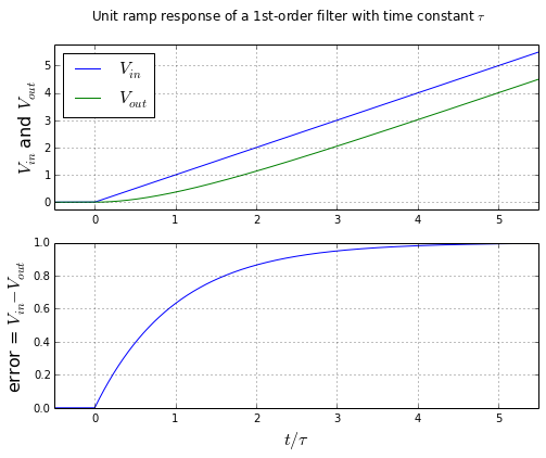
There's not zero steady-state error any more. This 1st-order system isn't good enough to follow a ramp with zero error. If we go back to the differential equation \( \frac{dV_{out}}{dt} = \frac{V_{in} - V_{out}}{\tau} \) and multiply both sides by τ we get \( V_{in}-V_{out} = \tau\frac{dV_{out}}{dt} \). In other words, the output can follow the ramp rate R of the input, but in order to do so, it has to have steady state error of \( \tau\frac{dV_{out}}{dt} = \tau R \). The slower the filter, the larger the steady-state error.
Sinusoidal input
The case of a sinusoidal input is mildly interesting. Rather than give the closed-form solution at first, let's use trapezoidal integration to simulate the response.
f = 0.3
Vin = (t>0)*np.sin(2*np.pi*f*t)
Vout = np.zeros_like(Vin)
y = Vout[0]
for i in range(1,len(Vout)):
    x = Vin[i]
    dt = t[i]-t[i-1]
    dy_dt_1 = (x-y)/tau
    y1 = y + dy_dt_1*dt
    dy_dt_2 = (x-y1)/tau
    y = y + (dy_dt_1 + dy_dt_2)*dt/2
    Vout[i] = y

ploterror(t,Vin,Vout,
 'Response to $\sin\, 2\pi ft$ with f=0.5'
 +' of a 1st-order filter with time constant $\\tau$')
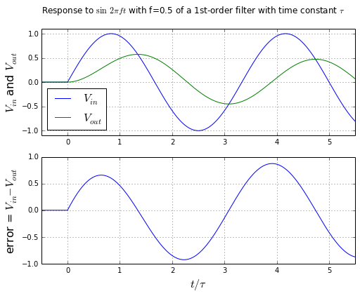
At "steady state" (there really isn't a true steady-state here) the following error is sinusoidal. Here we can use complex exponentials to help us. If our input is constant frequency, e.g. \( s=j2\pi f \,\Rightarrow\, V_{in} = e^{j2\pi ft} \), then the output is \( \frac{1}{\tau s+1}V_{in} \, \Rightarrow\, V_{out}=\frac{1}{1+j2\pi f\tau}e^{j2\pi ft} \), and that means that the steady-state error \( V_{in}-V_{out} = \left(1 - \frac{1}{1+j2\pi f\tau}\right) V_{in} \):
# ho hum, more Python code...

xlim = [-1.5,1.5]
alpha = np.logspace(xlim[0],xlim[1],300)
lxlim = [omega[0],alpha[-1]]
errfunc = lambda alpha: 1 - 1/(1j*alpha+1)
Hfunc = lambda alpha: 1/(1j*alpha+1)
db = lambda x: 20*np.log(np.abs(x))
ang = lambda x: np.angle(x,deg=True)
H = Hfunc(alpha)
err = errfunc(alpha)
axlist = []

fig = plt.figure(figsize=(8,6))
ax = fig.add_subplot(3,1,1)
ax.semilogx(alpha,db(H))
ax.set_ylabel(r'$\log |H(\omega)|$', fontsize=16)
#ax.set_ylim(1.05*ylim[0]-0.05*ylim[1],1.05*ylim[1]-0.05*ylim[0])
axlist.append(ax)

ax = fig.add_subplot(3,1,2)
ax.semilogx(alpha,ang(H))
yt=np.arange(np.min(ang(H))//15*15,np.max(ang(H))+15,15)
ax.set_yticks(yt)
ax.set_ylabel(r'$\measuredangle H(\omega)$',fontsize=16)
axlist.append(ax)


ax = fig.add_subplot(3,1,3)
ax.semilogx(alpha,db(err))
ax.set_ylabel(r'$\log |\tilde{H}(\omega)|$', fontsize=16)
#ax.set_ylim(1.05*ylim[0]-0.05*ylim[1],1.05*ylim[1]-0.05*ylim[0])
ax.set_xlabel(r'$ \alpha = 2\pi f\tau$',fontsize=16)
axlist.append(ax)

for (i,ax) in enumerate(axlist):
    ax.grid('on')
    ax.set_xlim(min(omega),max(omega))
    if i < 2:
        ax.set_xticklabels([])
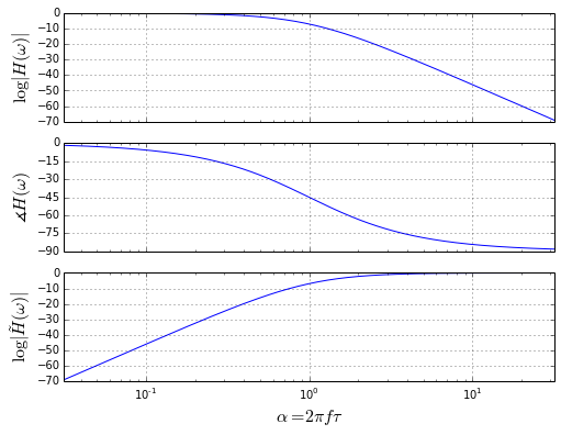
Here the critical quantity is \( \alpha = 2\pi f \tau \). We can quantify the input-to-output gain, phase lag, and error magnitude as a function of α. The exact values are input-to-output gain \( |H| = \frac{1}{\sqrt{1+\alpha^2}} \), phase lag \( \phi_{lag} =\measuredangle H = -\arctan \alpha \), and error magnitude \( |\tilde{H}| = \frac{\alpha}{\sqrt{1+\alpha^2}} \).
You can see the general behavior of these values in the graphs above.
For \( \alpha \ll 1 \), the input-to-output gain \( |H| \approx 1 - \frac{1}{2}\alpha^2 \); the phase lag in radians \( \phi_{lag} \approx -\alpha \), and the error magnitude \( |\tilde{H}| \approx \alpha \).
For \( \alpha \gg 1 \), the input-to-output gain \( |H| \approx \frac{1}{\alpha} \); the phase lag in radians \( \phi_{lag} \approx \frac{\pi}{2}-\frac{1}{\alpha} \), and the error magnitude \( |\tilde{H}| \approx 1 - \frac{1}{2 \alpha^2} \).
Wrapup
That's really it. All first-order systems are essentially alike. If you remove the constant term b, they are exactly alike and can be graphed with the same shape: the magnitude can be normalized by dividing by the gain term a, the time can be normalized by dividing by the time constant τ, and the frequency can be normalized by multiplying by the time constant τ.
The time response is exponential, and the frequency response contains one pole and, if the constant term b is present, one zero.
The steady-state error for a tracking first-order system \( H(s) = \frac{1}{\tau s + 1} \) is zero for a unit step, τ for a unit ramp, and has frequency-dependent behavior (see above) for sinusoidal inputs.
Not very interesting.
Things get more interesting when we get to higher-order systems. I'll talk about second-order systems in a future article.
© 2014 Jason M. Sachs, all rights reserved.


- Comments
- Write a Comment Select to add a comment
To post reply to a comment, click on the 'reply' button attached to each comment. To post a new comment (not a reply to a comment) check out the 'Write a Comment' tab at the top of the comments.
Please login (on the right) if you already have an account on this platform.
Otherwise, please use this form to register (free) an join one of the largest online community for Electrical/Embedded/DSP/FPGA/ML engineers: