Second-Order Systems, Part I: Boing!!

• Control Systems
• Applied Math
• Signal Processing

I’ve already written about the unexciting (but useful) 1st-order system, and about slew-rate limiting. So now it’s time to cover second-order systems.

The most common second-order systems are RLC circuits and spring-mass-damper systems.

Spring-mass-damper systems are fairly common; you’ve seen these before, whether you realize it or not. One household example of these is the spring doorstop (BOING!!):

(For what it’s worth: the spring doorstop appears to have been invented by Frank H. Chase during World War I.)

The mechanical systems may be more fun. But the electrical circuits are more relevant to embedded systems, so let’s start there.

Differential equations

Consider a series LRC circuit:

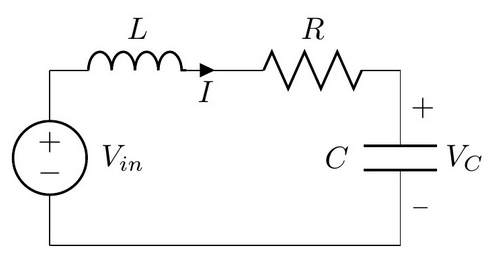
The equations for this system are

$$ \begin{aligned} C\frac{dV_C}{dt}&=I, \cr L\frac{dI}{dt}&=V_{in}-V_C-IR \end{aligned} $$

(Incidentally, I made that diagram with a short snippet of circuitikz. LaTeX and tikz are kind of quirky but once you get past the initial learning curve, you can get some really nice results.)

If you solve these equations for \( V_C \), you get

$$ LC\frac{d^2V_C}{dt}+RC\frac{dV_C}{dt}+V_C=V_{in} $$

The time-domain derivative operator \( \frac{d}{dt} \) is isomorphic to multiplication by the Laplace domain variable s, so in the Laplace domain, we have

$$H(s) = \frac{V_C}{V_{in}} = \frac{1}{LCs^2 + RCs + 1}$$

Hey, look! It’s a second-order system with a DC gain of 1. What else can we figure out about this system?

There are two standard forms of this type of second-order system, depending on whether you want to think of the timescale in terms of a time constant or a natural frequency:

$$H(s) = \frac{1}{\tau^2s^2 + 2\zeta\tau s + 1} = \frac{{\omega_n}^2}{s^2 + 2\zeta\omega_n s + {\omega_n}^2}$$

With our LRC circuit, this gives us \( \tau = \sqrt{LC} \), \( \omega_n = \frac{1}{\sqrt{LC}} \) and \( \zeta = \frac{R}{2}\sqrt{\frac{C}{L}} \).

The reason we put the transfer function into this form is because we can normalize the system response and scale the Laplace frequency to define \( \bar{s} = \tau s = s/\omega_n \):

$$H(\bar{s}) = \frac{1}{\bar{s}^2 + 2\zeta\bar{s} + 1}$$

This leaves only one parameter ζ. Second order systems with a constant numerator in the transfer function (no zeros) have a behavior that is completely determined by a timescale (natural frequency \( \omega_n \) or time constant τ) and damping factor (\( \zeta \)). Let’s forget about the damping factor for a moment, and just take a look at how the system response varies with \( \omega_n \):

import numpy as np
import matplotlib.pyplot as plt
from scipy.signal import lti, lsim, step

zeta = 0.456
t = np.arange(0,10,0.01)
wn_range = [1,2,5]
for wn in wn_range:
    H = lti([wn*wn],[1,2*zeta*wn,wn**2])
    t,y = H.step(T=t)
    plt.plot(t,y)
plt.xlabel('t')
plt.ylabel('step response')
plt.legend(['$\\omega_n = %.1f$' % wn for wn in wn_range],
           'lower right', fontsize=16)

 

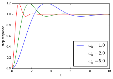
Same shape, different time scale. If we normalize the time scale \( \bar{t} = \omega_n t \), we get this:

zeta = 0.456
wn_range = [1,2,5]
for wn in wn_range:
    H = lti([wn*wn],[1,2*zeta*wn,wn**2])
    t,y = H.step()
    plt.plot(wn*t,y)
plt.xlabel('$\\bar{t} = \\omega_n t$',fontsize=16)
plt.ylabel('step response')
plt.legend(['$\\omega_n = %.1f$' % wn for wn in wn_range],
           'lower right', fontsize=16)

 

Hey, great! It’s just like first-order systems: the natural frequency \( \omega_n \) is not an interesting parameter. All systems with the same damping factor but different values of \( \omega_n \) are exactly the same, just with different time scales.

Damping factor

So let’s focus on the damping factor ζ and choose a fixed value for the natural frequency. We’ll choose \( \omega_n = 2\pi \) and look what happens for different values of ζ:

zeta_range = [0.1, 0.2, 0.3, 0.5, 0.7, 1.000001, 1.2, 1.5, 2.0]
wn = 2*np.pi
t = np.arange(0,4,0.005)
n = len(t)
plt.figure(figsize=(8,6))
hlines = []
for k, zeta in enumerate(zeta_range):
    H = lti([wn*wn],[1,2*zeta*wn,wn**2])
    _,y = H.step(T=t)
    hlines.append(plt.plot(t,y))
    if zeta >= 1:
        klbl = int(n * 0.12) 
        tl = t[klbl]
        yl = y[klbl]
    else:
        zcomp = np.sqrt(1-zeta**2)
        wd = zcomp*wn
        tl = np.pi/wd
        yl = 1+np.exp(-np.pi*zeta/zcomp)
    plt.annotate('$\\zeta=%.3f$' % zeta, xy=(tl,yl), xytext=(-0.45,yl),
        xycoords='data', textcoords='data',
        arrowprops=dict(arrowstyle="-", shrinkB=0),
        verticalalignment='top',
        fontsize=13
        )
for k, zeta in enumerate ([z for z in zeta_range if z < 0.5]):
    A = 1/np.sqrt(1-zeta**2)
    hl2 = plt.plot(t,1+A*np.exp(-zeta*wn*t), '--',
                   t,1-A*np.exp(-zeta*wn*t), '--')
    for hl in hl2:
        hl.set_color(hlines[k][0].get_color())
        hl.set_linewidth(hlines[k][0].get_linewidth()*0.4)
plt.xlim([-0.5,4])
plt.ylim([0,1.8])
plt.xlabel('t')
plt.title('Second-order system step response for '
          +'$\\omega_n = 2\\pi$, '
          +'different damping factors'
          )

 

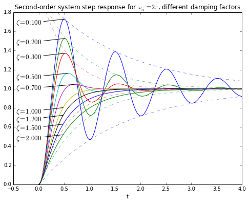
Values of ζ that are less than 1.0 lead to underdamped systems, which have an overshoot. Values of ζ that are greater than 1.0 lead to overdamped systems, which do not have an overshoot, and which settle more slowly. If ζ = 1.0 then the system is critically damped; this is the minimum value for ζ that does not have an overshoot.

How do we figure out the overshoot as a function of ζ ?

Poles and Overshoot

Let’s look again at the denominator of the transfer function, \( s^2 + 2\zeta\omega_n s + {\omega_n}^2 \). If we factor it, we can find the poles of the transfer function. So solve for \( s^2 + 2\zeta\omega_n s + {\omega_n}^2 = 0 \) using the quadratic formula:

$$ s = \frac{-2\zeta\omega_n \pm \sqrt{4\zeta^2{\omega_n}^2 - 4{\omega_n}^2} }{2} = \omega_n\left(-\zeta \pm \sqrt{\zeta^2 - 1}\right) $$

If \( \zeta > 1 \), both poles are real and the equation tells us how to compute them. (For example, if \( \zeta = 1.6 \), then the poles are at \( s=-0.351\omega_n \) and \( s=-2.849\omega_n \).)

If \( \zeta = 1 \), then both poles are at \( s=-\omega_n \).

If \( \zeta < 1 \) — the underdamped case — then the poles are a complex conjugate pair at \( s = \omega_n\left(-\zeta \pm j\sqrt{1-\zeta^2}\right) = -\alpha \pm j\omega_d \) where \( \alpha = \zeta\omega_n \) is the decay rate and \( \omega_d = \omega_n\sqrt{1-\zeta^2} \) is the damped natural frequency.

The underdamped case is the most interesting one. We can solve for the step response \( h_1(t) \) and impulse response \( h(t) = \frac{d}{dt}h_1(t) \) exactly; if you go through the grungy math, it turns out that

$$ \begin{aligned} h(t) &= u(t) \frac{\omega_n}{\sqrt{1-\zeta^2}} e^{-\alpha t} \sin \omega_d t \cr h_1(t) &= u(t) \left(1-\frac{\zeta}{\sqrt{1-\zeta^2}} e^{-\alpha t} \sin \omega_d t - e^{-\alpha t}\cos\omega_d t\right) \cr &= u(t) \left(1+\frac{1}{\sqrt{1-\zeta^2}} e^{-\alpha t} \sin (\omega_d t + \phi)\right) \end{aligned} $$

which is not too complicated. The nice thing is that we can make a couple of conclusions here:

1. At t = 0, the slope of the step response is zero. (In our LCR circuit, that’s because the rate of change in output voltage \( \frac{dV_C}{dt} = I/C \), and the inductor current starts off at zero.)

2. The local extrema (the points that are a local minimum or maximum) of the step response are the instants where its derivative (= the impulse response) is zero, which occurs when \( \sin \omega_d t = 0 \), namely at integer multiples of \( \frac{T}{2} = \frac{\pi}{\omega_d} \).

3. The point of maximum overshoot is the first extremum after \( t=0 \), and occurs at \( t=\frac{\pi}{\omega_d} \). For our example with \( \omega_n=2\pi \), at low values of ζ this occurs at t=0.5; as ζ increases, the damped natural frequency slows down a little bit.

4. The value of maximum overshoot is pretty easy to calculate; we just plug in \( t=\frac{\pi}{\omega_d} \), and since \( \sin\omega_d t = 0 \) there, we are left with

$$ h_1(t) = 1- e^{-\alpha t}\cos\omega_d t = 1+e^{-\alpha \frac{\pi}{\omega_d}}$$

and therefore the overshoot is the amount this exceeds 1.0, which is

$$ OV = e^{-\alpha \frac{\pi}{\omega_d}} = e^{-\pi \frac{\zeta}{\sqrt{1-\zeta^2}}}$$

zeta = np.arange(0.001,0.999,0.001)
plt.plot(zeta,np.exp(-np.pi*zeta/np.sqrt(1-zeta**2)))
plt.xlabel('$\zeta$',fontsize=15)
plt.ylabel('overshoot',fontsize=12)
plt.grid('on')

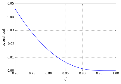
zeta = np.arange(0.7,0.999,0.001)
plt.figure()
plt.plot(zeta,np.exp(-np.pi*zeta/np.sqrt(1-zeta**2)))
plt.xlim(0.7,1)
plt.xlabel('$\zeta$',fontsize=15)
plt.ylabel('overshoot',fontsize=12)
plt.grid('on')

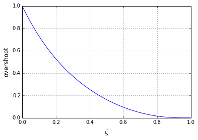
If we want to solve this equation for the damping factor, we get \( \zeta = \sqrt{\frac{(\ln OV)^2}{\pi^2 + (\ln OV)^2}} \)

Note that the overshoot decreases rapidly with increasing ζ, and once you reach about ζ = 0.7, the overshoot is small and decreases more slowly. That’s an important factor for system design. Let’s say you are tuning a system and need to trade off the value of ζ against other design choices. If you can tolerate a small amount of overshoot, and your design tradeoffs would benefit from a smaller value of ζ, you don’t need an overdamped system; you can generally tolerate a ζ in the range of 0.7 - 0.9.

Summary and what’s next

We looked at second order systems of the form

$$H(s) = \frac{1}{\tau^2s^2 + 2\zeta\tau s + 1} = \frac{{\omega_n}^2}{s^2 + 2\zeta\omega_n s + {\omega_n}^2}$$

and examined features of the step response. This transfer function has a DC gain of 1, two poles, and no zeroes. Its timescale is determined by the natural frequency \( \omega_n \) and its shape is determined by the damping factor ζ. Systems with \( \zeta < 1 \) are underdamped and have two conjugate poles. Systems with \( \zeta > 1 \) are overdamped and have two real poles.

Other characteristics of the step response:

• The poles are located at \( s=\omega_n\left(-\zeta \pm \sqrt{\zeta^2 - 1}\right) \) for overdamped systems and \( s=\omega_n\left(-\zeta \pm j\sqrt{1-\zeta^2}\right) \) for underdamped systems.
• For underdamped systems:
  • the step response looks like \( 1 + \frac{1}{\sqrt{1-\zeta^2}}e^{-\alpha t} \sin(\omega_d t + \phi) \)
  • the envelope of the step response decays with a rate of \( \alpha = \zeta\omega_n \)
  • the resonance occurs at \( \omega_d = \omega_n\sqrt{1-\zeta^2} \)
  • the overshoot is equal to \( OV = e^{-\alpha \frac{\pi}{\omega_d}} = e^{-\pi \frac{\zeta}{\sqrt{1-\zeta^2}}} \)

In Part II we’ll look at how the presence of a zero affects the behavior of second-order systems.

© 2014 Jason M. Sachs, all rights reserved.

Sign in