The Power Spectrum

Often, when calculating the spectrum of a sampled signal, we are interested in relative powers, and we don’t care about the absolute accuracy of the y axis.  However, when the sampled signal represents an analog signal, we sometimes need an accurate picture of the analog signal’s power in the frequency domain.  This post shows how to calculate an accurate power spectrum.

Parseval’s theorem [1,2] is a property of the Discrete Fourier Transform (DFT) that states:

$$\sum_{n=0}^{N-1} |x(n)|^2 = \frac1N\sum_{k=0}^{N-1}|X(k)|^2$$

where

• x(n) is a time sequence (real or complex)
• X(k) is the discrete Fourier transform of x(n)
• n = 0:N-1 is the time index of x
• k = 0:N-1 is the frequency index of X

Multiply both sides of the above by 1/N:

$$\frac1N\sum_{n=0}^{N-1} |x(n)|^2 = \frac1{N^2}\sum_{k=0}^{N-1}|X(k)|^2$$

|x(n)|² is the instantaneous power of a sample of the time signal into a 1-ohm load.  So the left side of the equation is just the average power of the signal over the N samples.  Thus, for a 1-ohm load,

$$P_{av}= \frac1{N^2}\sum_{k=0}^{N-1}|X(k)|^2  \quad{watts}$$

For the each DFT bin, we can say:

$$P_{bin}(k)= \frac1{N^2}|X(k)|^2, \quad{k=0:N-1}  \quad{watts/bin}\quad{(1)}$$

This is the power spectrum of the signal.  For a load resistance R, just divide equation 1 by R.

Note that X(k) is the two-sided spectrum.  If x(n) is real, then X(k) is symmetric about f_s/2, with each side containing half of the power.  In that case, we can choose to keep just the one-sided spectrum, and multiply P_bin by 2:

$$P_{bin}(k) \quad{one-sided} = \frac2{N^2}|X(k)|^2, \quad{k=0:N/2-1}  \quad{watts/bin}\quad{(2)}$$

Here are a couple of examples that compute the power spectra for sinusoidal signals.

Example 1.  Power spectrum of a sinusoid with frequency at FFT bin center.

Let x = A*sin(2πf_cnT_s), with A = sqrt(2), fc = 5 Hz,  f_s = 1/T_s = 32 Hz, and N = 32.  The power into 1 ohm of the analog version of this sinusoid is A²/2 = 1 watt.

Here is the Matlab code to compute the power spectrum:

% power_spectrum1.m
fs= 32;                     % Hz  sample rate
N= 32;
fc= 5;                      % Hz freq of sine wave
n= 0:N-1;
t= n/fs;                    % s
A= sqrt(2);                 % Volts
x= A*sin(2*pi*fc*t);        % time signal
% Compute Power Spectrum
k= 0:N-1;                   % freq index
f= k*fs/N;                  % Hz
X= fft(x);
Pbin= abs(X).^2/N^2;        % watts/bin  power spectrum
% Plot 2-sided spectrum
stem(f,Pbin),grid
axis([0 fs 0 .6]);
xlabel('Hz'),ylabel('Watts'),figure
Pdisplay= 2*Pbin(1:N/2);    % one-sided spectrum watts/bin
% Plot one-sided spectrum
stem(f(1:N/2),Pdisplay),grid
axis([0 fs/2 0 1.1]);
xlabel('Hz'),ylabel('Watts')

The two-sided and one-sided spectra for this (very simple) example are shown below.  As expected, the one-sided plots shows a power of 1 watt at f = 5 Hz.

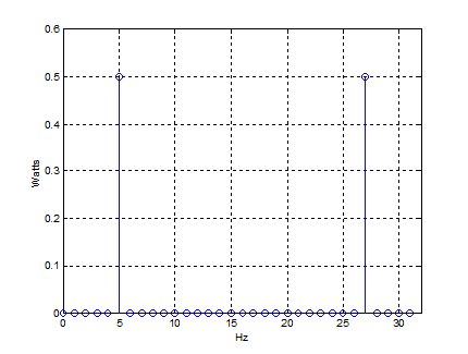
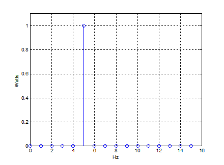
Figure 2.  One-sided power spectrum

Example 2.  Power spectrum of two sinusoids – one at FFT bin center and one between bins.

Let x = A*sin(2πf₁nT_s) + A* sin(2πf₂nT_s), with A = sqrt(2), f₁ = 125 Hz, f2 = 135.25 Hz, f_s = 1/T_s = 1024 Hz, and N = 2048. 

The power into 1 ohm of the analog version of each sinusoidal component is A²/2 = 1 watt.  The component at 125 Hz falls on a bin center, while the component at 135.25 Hz falls between the bins (bin spacing is 1024 Hz/2048 = 0.5 Hz).

To prevent spectral leakage of the component at 135.25 Hz, we apply a window [3,4,5] to the time sequence.  To preserve power accuracy, we need to normalize the window function’s power to 1.  Given window function w(n), we multiply by a constant C such that:

$$\frac1{N}\sum_{n=0}^{N-1}(Cw(n))^2  = 1$$

Solving for C, we get:

$$C= \sqrt{ \frac N{\sum_{n=0}^{N-1}(w(n))^2} }$$

Here is the Matlab code to compute the power spectrum.  It includes a normalized Hanning window.

% power_spectrum2.m     10/7/16 nr
% Plot the power spectrum of two sines with amplitude of sqrt(2) volts.
% P = A^2/2 = 1 watt.
% one sine frequency is in center of bin and one is between bins
% use hanning window
fs= 1024;                  % Hz  sample frequency
N= 2048;
f1= 125;                   % Hz f1 falls on bin-center
f2= 135.25;                % Hz f2 falls between bins
n= 0:N-1;                  % time index
t= n/fs;                   % s
A= sqrt(2);                % Volts
x= A*sin(2*pi*f1*t) + A*sin(2*pi*f2*t);      % time signal
w= hanning(N)';            % hanning window
w= w.*sqrt(N/sum(w.^2));   % normalize window for P= 1;
xw= x.*w;                  % multiply signal by window
% Compute Power Spectrum
k= 0:N/2 -1;               % freq index of one-sided spectrum
f= k*fs/N;                 % Hz
X= fft(xw);
Pbin= 2*abs(X(1:N/2)).^2/N^2;         % W/bin factor of 2 for one-sided spectrum
PbindB= 10*log10(abs(Pbin));
plot(f,PbindB,'.-'),grid
axis([115 145 -50 5])
xlabel('Hz'),ylabel('dBW')

The one-sided spectrum plotted around the signal frequencies is shown in Figure 3.  Why are the peaks not at 0 dBW (1 watt)?  Windowing in time causes each of our two spectral components to be convolved with the spectrum of the window.  The power is thus spread out over the window’s bandwidth, so the peak is less than the total power.  To compute the power of each component, we have to sum the power over the window’s bandwidth.  In the code below, we have summed the power of the frequency sample at f₁ and 2 samples on either side; likewise for f₂.    The result is plotted in Figure 4 as the red circles, which show 0 dBW at each frequency.

We should also note that the scalloping effect of the Hanning window is visible – the peak at 135.25 Hz is 1.42 dB below that at 125 MHz.  Although this scalloping has not harmed the power calculation, it is visually somewhat confusing.  Note the scalloping could be reduced by zero-padding the windowed time signal, but this has not been done here [6].

Finally, these examples have used sinusoids, which are deterministic signals.  To display the spectra of random signals, we would need to add FFT-averaging to the techniques discussed here.

% Post-Processing
% Compute power of components at f1 and f2
k1= round(f1*N/fs);        % index of f1
P1= sum(Pbin(k1-2:k1+2))   % W    sum of spectrum components around f1
P1dB= 10*log10(P1);        % dBW
k2= round(f2*N/fs);        % index of f2
P2= sum(Pbin(k2-2:k2+2))   % W    sum of spectrum components around f2
P2dB= 10*log10(P2);        % dBW
plot(f,PbindB,'.-',[f1 f2],[P1dB P2dB],'or'),grid
axis([115 145 -50 5])
xlabel('Hz'),ylabel('dBW')

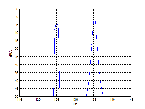
Figure 3.  Power Spectrum of sinusoids using windowing. 

                   Peaks are lower than the actual power of 0 dBW.

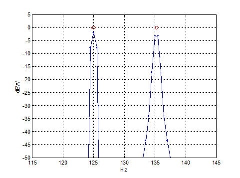
Figure 4.  Power Spectrum of sinusoids using windowing. 

Red circles = Power of each spectral component

References

1.  Sanjit K. Mitra, Digital Signal Processing (2^nd Ed), McGraw-Hill, 2001, Table 3.5.

2.  https://en.wikipedia.org/wiki/Parseval%27s_theorem, subsection Notation Used in Engineering and Physics.

3.  Richard G. Lyons, Understanding Digital Signal Processing (2^nd Ed) , Prentice Hall, 2004, Section 3.9.

4.  https://en.wikipedia.org/wiki/Window_function

5.  Segio Rapuano and Fred J. Harris, “An Introduction to FFT and Time Domain Windows”, IEEE Instrumentation and Measurement Magazine, Dec 2007, p. 32.

6.  Lyons, sections 3.10, 3.11.

Oct 8, 2016  Neil Robertson

Sign in