Simplest Calculation of Half-band Filter Coefficients

Half-band filters are lowpass FIR filters with cut-off frequency of one-quarter of sampling frequency f_s and odd symmetry about f_s/4  [1]*.  And it so happens that almost half of the coefficients are zero.  The passband and stopband bandwiths are equal, making these filters useful for decimation-by-2 and interpolation-by-2.  Since the zero coefficients make them computationally efficient, these filters are ubiquitous in DSP systems.

Here we will compute half-band coefficients using the window method.  While the window method typically does not yield the fewest taps for a given performance, it is useful for learning about half-band filters.  Efficient equiripple half-band filters can be designed using the Matlab function firhalfband [2].

Coefficients by the Window Method

The impulse response of an ideal lowpass filter with cut-off frequency ω_c = 2πf_c/f_s is [3]:

$$h(n)=\frac{sin(\omega_c n)}{\pi n}, \quad -\infty < n < \infty $$

This is the familiar sinx/x or sinc function (scaled by ω_c/π).  To create a filter using the window method, we truncate h(n) to N+1 samples and then apply a window.  For a halfband filter, ω_c = 2π*1/4 = π/2.  So the truncated version of h(n) is:

$$h(n)=\frac{sin(n\pi /2)}{n\pi}, \quad -N/2 < n < N/2 $$

Now apply a window function w(n) of length N+1 to obtain the filter coefficients b:

$$b(n)=h(n)w(n), \quad -N/2 < n < N/2 $$

$$b(n)=\frac{sin(n\pi /2)}{n\pi}w(n), \quad -N/2 < n < N/2 \qquad (1)$$

Choice of a particular window function w(n) is based on a compromise between transition bandwidth and stopband attenuation.  As a simple example, the Hamming window function of length N+1 is**:

$$w(n)= 0.54+0.46cos(\frac{2\pi n}{N}),\quad -N/2 < n < N/2 $$

And that’s it!  Equation 1 is all you need to compute the coefficients.  Note that N is even and the filter length is N+1 (odd length).  

Examples using Matlab

Here is Matlab code that implements Equation 1 for ntaps = 19:

ntaps= 19;
N= ntaps-1;
n= -N/2:N/2;
sinc= sin(n*pi/2)./(n*pi+eps);      % truncated impulse response; eps= 2E-16
sinc(N/2 +1)= 1/2;                  % value for n --> 0
win= kaiser(ntaps,6);               % window function
b= sinc.*win';

I used the Matlab Kaiser window function b= kaiser(ntaps,beta), where beta determines the sidelobe attenuation in the frequency domain [5].  Higher beta gives better stopband attenuation in the halfband filter, at the expense of wider transition band.  Figure 1 shows the truncated sinc function, the window function, and the coefficients.  Every other coefficient is zero, except for the main tap.  This follows from the fact that every other sample of the truncated sinc function is zero.  The scale of the plot obscures the values of the end coefficients; b(-9) and b(9) are equal to .000526. 

Figure 2 shows the magnitude response for f_s= 100 Hz, with a linear amplitude scale.  The response of the ideal lowpass filter is also shown.  The amplitude is 0.5 at f_s/4 = 25 Hz.  Note the odd symmetry with respect to (x,y) = (25, 0.5).

As already mentioned, ntaps must be odd.  It is possible to create a halfband frequency response with ntaps even, but in that case, there will be no zero-valued coefficients.  Also, for ntaps = 9, 13, … etc, the end coefficients are zero.  For this reason, we should choose ntaps = 4m + 3, where m is an integer.  Thus the useful values of ntaps are 7, 11, 15, etc.  The number of zero coefficients is ½(ntaps-3).

Now let’s look at the response for different values of ntaps (Figure 3).  The upper graph uses a linear amplitude scale, while the lower one uses dB.  As you can see, the stopband attenuation does not change much vs. ntaps, but the transition band becomes sharper as ntaps is increased.  The trade-off between attenuation and transition band can be changed by adjusting the Kaiser window’s beta value.

Footnotes

*  Mathematically, $H(e^{jω}) + H(e^{j(π-ω)})  = 1 $ , where ω = 2πf/f_s.

**  If we let n = 0:N instead of –N/2:N/2, the expression for the Hamming window is [4]:

$$w(n)= 0.54-0.46cos(\frac{2\pi n}{N}),\quad  n= 0:N $$

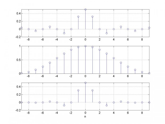
 Figure 1.  Coefficients of Halfband Filter with ntaps = 19

top:  Truncated sinc function     center:  Kaiser window with beta = 6     bottom:  Filter coefficients

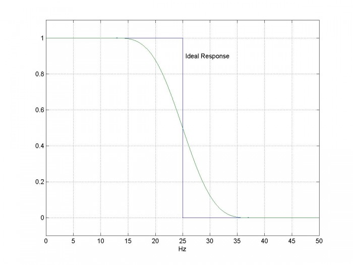
Figure 2.  Magnitude response of halfband filter with ntaps = 19, f_s= 100 Hz (linear amplitude scale)

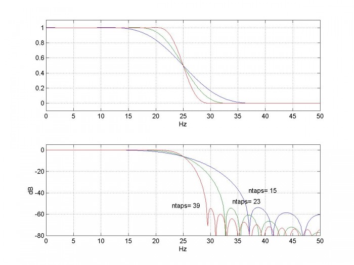
Figure 3.  Halfband filter magnitude response for different length filters, f_s = 100 Hz

                top:  linear amplitude scale             bottom:  dB amplitude scale

Other DSPRelated.com Posts on Halfband filters

Here are a couple of other posts about halfband filters on DSPRelated.com:

Rick Lyons, “Optimizing the Half-band Filters in Multistage Decimation and Interpolation”, Jan 2016.  https://www.dsprelated.com/showarticle/903.php

Christopher Felton, “Halfband Filter Design with Python/Scipy, Feb 2012. https://www.dsprelated.com/showcode/270.php

References

1.  Sanjit K. Mitra, Digital Signal Processing, 2^nd Ed., McGraw-Hill, 2001, p 701-702.

2.  Mathworks website https://www.mathworks.com/help/dsp/ref/firhalfband.html

3.  Mitra, p 448.

4.  Mathworks website https://www.mathworks.com/help/signal/ref/hamming.html

5.  Mathworks website https://www.mathworks.com/help/signal/ref/kaiser.html

Neil Robertson   November, 2017

Appendix  A   Matlab Function for Halfband Filter Coefficients

This program is provided as-is without any guarantees or warranty.  The author is not responsible for any damage or losses of any kind caused by the use or misuse of the program.

%hbsynth.m       11/13/17 Neil Robertson
% Halfband filter synthesis by the window method, using a Kaiser window.
% input argument ntaps must be odd.
function b= hbsynth(ntaps)
if mod(ntaps,2)==0
   error('  ntaps must be odd')
end
N= ntaps-1;
n= -N/2:N/2;
sinc= sin(n*pi/2)./(n*pi+eps);      % truncated impulse response; eps= 2E-16
sinc(N/2 +1)= 1/2;                  % value for n --> 0
win= kaiser(ntaps,6);               % window function
b= sinc.*win';                      % apply window function

Appendix B   Matlab Code to Create Figure 3

%hb_ex1.m    11/13/17 Neil Robertson
fs= 100;
b1= hbsynth(15);
b2= hbsynth(23);
b3= hbsynth(39);
[h1,f]= freqz(b1,1,512,fs);
H1= 20*log10(abs(h1));
[h2,f]= freqz(b2,1,512,fs);
H2= 20*log10(abs(h2));
[h3,f]= freqz(b3,1,512,fs);
H3= 20*log10(abs(h3));
subplot(211),plot(f,abs(h1),f,abs(h2),f,abs(h3)),grid
axis([0 fs/2 -.1 1.1]),xlabel('Hz')
subplot(212),plot(f,H1,f,H2,f,H3),grid
axis([0 fs/2 -80 5]),xlabel('Hz'),ylabel('dB')
text(37,-38,'ntaps= 15')
text(34,-48,'ntaps= 23')
text(23,-52,'ntaps= 39')

Sign in