Design IIR Bandpass Filters

In this post, I present a method to design Butterworth IIR bandpass filters.  My previous post [1] covered lowpass IIR filter design, and provided a Matlab function to design them.  Here, we’ll do the same thing for IIR bandpass filters, with a Matlab function bp_synth.m.  Here is an example function call for a bandpass filter based on a 3^rd order lowpass prototype:

N= 3;             % order of prototype LPF
fcenter= 22.5;    % Hz  center frequency, Hz
bw= 5;            % Hz  -3 dB bandwidth, Hz
fs= 100;          % Hz  sample frequency
[b,a]= bp_synth(N,fcenter,bw,fs)
b =  0.0029    0   -0.0087    0    0.0087    0   -0.0029
a =  1.0000   -0.8512    2.6169   -1.3864    2.1258   -0.5584    0.5321

There are seven “b” (numerator) and seven “a” (denominator) coefficients, so H(z) is 6^th order.  To find the frequency response:

[h,f]= freqz(b,a,512,fs);
H= 20*log10(abs(h));

The magnitude response of the filter is shown in Figure 1, along with the response of the equivalent analog bandpass filter.

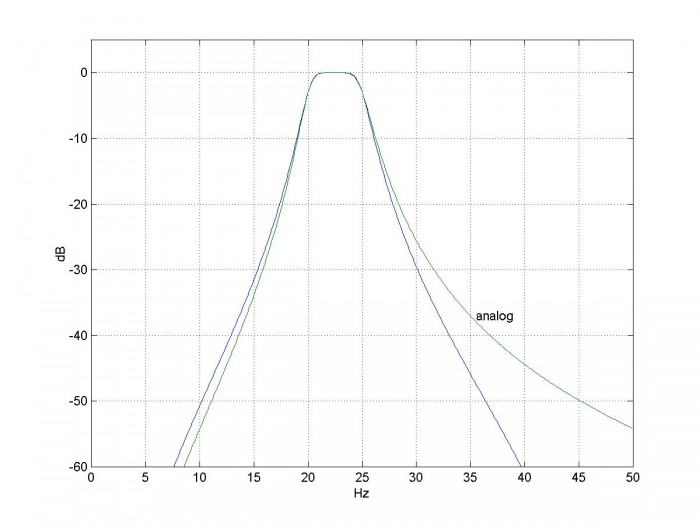
Figure 1.  Magnitude response of bandpass filter based on N= 3 lowpass prototype. 

fcenter=  22.5 Hz, bw= 5 Hz, and fs= 100 Hz.  The equivalent analog filter’s response is also shown.

Filter Synthesis

Here is a summary of the steps for computing the bandpass filter coefficients.  Recall from the previous post that F is continuous (analog) frequency in Hz and Ω is continuous radian frequency.

1. Find the poles of a lowpass analog prototype filter with Ω_c = 1 rad/s.
2. Given upper and lower -3 dB frequencies of the digital bandpass filter, find the corresponding frequencies of the analog bandpass filter (pre-warping).
3. Transform the analog lowpass poles to analog bandpass poles.
4. Transform the poles from the s-plane to the z-plane, using the bilinear transform.
5. Add N zeros at z= -1 and N zeros at z= +1, where N is the order of the lowpass prototype.
6. Convert poles and zeros to polynomials with coefficients a_n and b_n.

These steps are similar to the lowpass design procedure, with steps 2, 3, 5, and 6 modified for the bandpass case.  Now let’s look at the design procedure in detail.  A Matlab function bp_synth that performs the filter synthesis is provided in Appendix A.

1.  Poles of the analog lowpass prototype filter.  For a Butterworth filter of order N with Ω_c = 1 rad/s, the poles are given by [2,3]:

$$p'_{ak}= -sin(\theta)+jcos(\theta)$$

where $$\theta=\frac{(2k-1)\pi}{2N},\quad k=1:N$$

Here we use a prime superscript on p to distinguish the lowpass prototype poles from the yet to be calculated bandpass poles.

2.  Given upper and lower -3 dB frequencies of the digital bandpass filter, find the corresponding frequencies of the analog bandpass filter.  We define f_center as the center frequency in Hz, and bw_Hz as the -3 dB bandwidth in Hz.  Then the -3 dB discrete frequencies are :

$$f_1=f_{center}-bw_{Hz}/2$$

$$f_2=f_{center}+bw_{Hz}/2$$

As before, we’ll adjust (pre-warp) the analog frequencies to take the nonlinearity of the bilinear transform into account:

$$F_1=\frac{f_s}{\pi}tan\left(\frac{\pi f_1}{f_s}\right)$$

$$F_2=\frac{f_s}{\pi}tan\left(\frac{\pi f_2}{f_s}\right)$$

We need to define two more quantities:

 BW_Hz = F₂ – F₁ Hz is the pre-warped -3 dB bandwidth, and 

$F_0=\sqrt{F_1F_1}$ is the geometric mean of F1 and F2.  

3.  Transform the analog lowpass poles to analog bandpass poles.  See Appendix B for a derivation of the transformation.  For each lowpass pole p_a' , we get two bandpass poles:

$$p_a=2\pi F_0\left[\frac{BW_{Hz}}{2F_0}p'_a \pm j\sqrt{1-\left(\frac{BW_{Hz}}{2F_0}p'_a\right)^2}\ \right]$$

4.  Transform the poles from the s-plane to the z-plane, using the bilinear transform.  This is the same as for the IIR lowpass, except there are 2N instead of N poles:

$$p_k=\frac{1+p_{ak}/(2f_s)}{1-p_{ak}/(2f_s)},\quad k=1:2N$$

5.  Add N zeros at z= -1 and N zeros at z= +1.  See Appendix B for details.  We can now write H(z) as:

$$H(z)=K\frac{(z+1)^N(z-1)^N}{(z-p_1)(z-p_2)...(z-p_{2N})}\qquad(1)$$

In bp_synth, we represent the N zeros at -1 and N zeros at +1 as a vector:

     q= [-ones(1,N) ones(1,N)]

6.  Convert poles and zeros to polynomials with coefficients a_n and b_n.  If we expand the numerator and denominator of equation 1 and divide numerator and denominator by z^2N, we get polynomials in z^-n:

$$H(z)=K\frac{b_0+b_1z^{-1}+...+b_{2N}z^{-2N}}{1+a_1z^{-1}+...+a_{2N}z^{-2N}}$$

 The Matlab code to perform the expansion is:

     a= poly(p)
     a= real(a)
     b= poly(q)

We want H(z) to have a gain of 1 at f = f₀.  We can do this by evaluating H(z) at f₀ and setting K = 1/|H(f₀)|.  The Matlab code is:

     f0= sqrt(f1*f2);
     h= freqz(b,a,[f0 f0],fs);
     K= 1/abs(h(1));

Example

Here’s an example IIR bandpass filter based on a 2^nd order lowpass.  We’ll show the different poles and zeros computed by bp_synth.m.  (Note the pole and zero values are not printed by the code listed in Appendix A).  The function call is as follows:

N= 2;             % order of prototype LPF
fcenter= 20;      % Hz  center frequency, Hz
bw= 4;            % Hz  -3 dB bandwidth, Hz
fs= 100;          % Hz  sample frequency
[b,a]= bp_synth(N,fcenter,bw,fs)

Here are the pole and zero computed values.  Note Matlab uses an a+bi format for complex numbers.

Two poles of analog lowpass butterworth prototype with Ω’ = 1 rad/s

(p_lp is the same as p_a’):

  p_lp =  -0.7071 + 0.7071i  -0.7071 - 0.7071i

Four poles of analog bandpass:

  pa =  1.0e+002 *
  -0.1490+ 1.5854i  -0.1234+ 1.3130i  -0.1234- 1.3130i  -0.1490- 1.5854i

Four poles of IIR bandpass:

  p= 0.2053+ 0.8892i   0.3627+ 0.8426i   0.3627- 0.8426i   0.2053- 0.8892i

Two zeros at z= -1 and two zeros at z= 1:

  q =    -1    -1     1     1

The IIR bandpass poles and zeros are shown in Figure 2.  Now let’s look at the filter coefficients. 

Numerator coefficients before scaling:

  b =     1     0    -2     0     1

Numerator scale factor:

  K =    0.0134

Filter coefficients b and a:

  b =    0.0134         0   -0.0267         0    0.0134
  a =    1.0000   -1.1361    1.9723   -0.9498    0.7009

From K, b, and a we can write the filter’s transfer function:

$$H(z)=.0134*\frac{1-2z^{-2}+z^{-4}}{1-1.1361z^{-1}+1.9723z^{-2}-.9498z^{-3}+.7009z^{-4}}$$

The filter’s magnitude response is plotted as the N=2 curve in Figure 3.

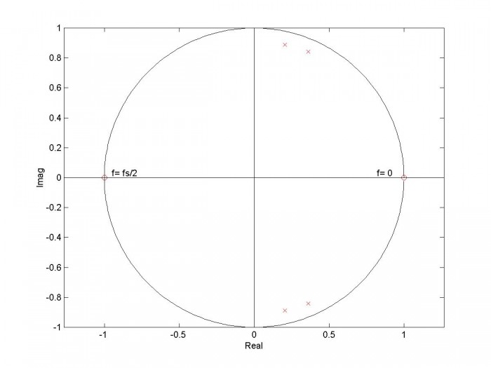
Figure 2.  Pole-zero plot of bandpass filter based on 2^nd order lowpass prototype.

                  fcenter= 20 Hz, bw= 4 Hz, and fs= 100 Hz.  Zeros at z= +/-1 are 2^nd order.

Filter Performance

As was the case for lowpass IIR filters, the bandpass IIR response has more rejection than that of the analog prototype as you approach f_s/2 (see Figure 1).  This is due to the bilinear transform, which compresses the entire bandwidth into 0 to f_s/2.  Thus, the analog zeros at infinity occur at f_s/2 for the discrete-time filter.

Figure 3 compares the magnitude response of bandpass filters based on 1^st, 2^nd, and 3^rd order Butterworth lowpass filters.  They all have the same -3 dB bandwidth of 4 Hz.  Figure 4 shows the group delay response of the same filters:  as you would expect for IIR filters, the group delay is not flat.

Caveats

Performance of IIR filters can be hurt by coefficient quantization and roundoff noise [4,5].  In particular, when the poles are close to the unit circle, quantization of the denominator coefficients can cause a pole to move outside the unit circle, making the filter unstable.  Bandpass filters with narrow bandwidth and higher order are most susceptible. 

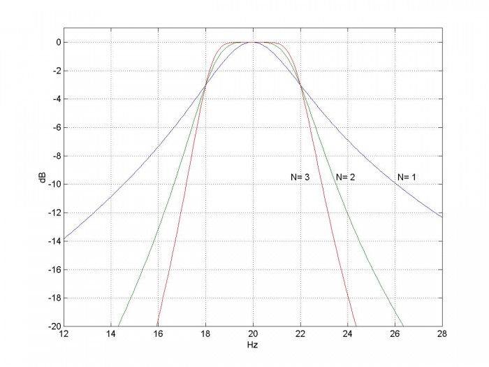
Figure 3.  Magnitude response of bandpass filters vs. order of lowpass prototype.

 fcenter= 20 Hz, bw= 4 Hz, and fs= 100 Hz.

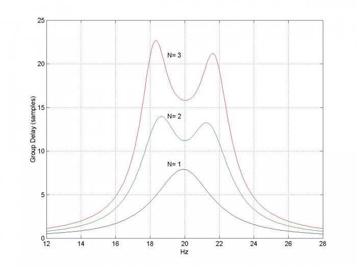
Figure 4.  Group Delay of bandpass filters vs. order of lowpass prototype.

 fcenter= 20 Hz, bw= 4 Hz, and fs= 100 Hz.  [gd,f]= grpdelay(b,a,512,fs);

Appendix A.  Matlab Function bp_synth

This program is provided as-is without any guarantees or warranty.  The author is not responsible for any damage or losses of any kind caused by the use or misuse of the program.

%function [b,a]= bp_synth(N,fcenter,bw,fs)      12/29/17 neil robertson
% Synthesize IIR Butterworth Bandpass Filters
%
% N= order of prototype LPF
% fcenter= center frequency, Hz
% bw= -3 dB bandwidth, Hz
% fs= sample frequency, Hz
% [b,a]= vector of filter coefficients
%
function [b,a]= bp_synth(N,fcenter,bw,fs)
f1= fcenter- bw/2;            % Hz lower -3 dB frequency
f2= fcenter+ bw/2;            % Hz upper -3 dB frequency
if f2>=fs/2;
   error('fcenter+ bw/2 must be less than fs/2')
end
if f1<=0
   error('fcenter- bw/2 must be greater than 0')
end
% find poles of butterworth lpf with Wc = 1 rad/s
k= 1:N;
theta= (2*k -1)*pi/(2*N);
p_lp= -sin(theta) + j*cos(theta);    
% pre-warp f0, f1, and f2
F1= fs/pi * tan(pi*f1/fs);
F2= fs/pi * tan(pi*f2/fs);
BW_hz= F2-F1;              % Hz prewarped -3 dB bandwidth
F0= sqrt(F1*F2);           % Hz geometric mean frequency
% transform poles for bpf centered at W0
% note:  alpha and beta are vectors of length N; pa is a vector of length 2N
alpha= BW_hz/F0 * 1/2*p_lp;
beta= sqrt(1- (BW_hz/F0*p_lp/2).^2);
pa= 2*pi*F0*[alpha+j*beta  alpha-j*beta];
% find poles and zeros of digital filter
p= (1 + pa/(2*fs))./(1 - pa/(2*fs));      % bilinear transform
q= [-ones(1,N) ones(1,N)];                % N zeros at z= -1 (f= fs/2) and z= 1 (f = 0)
% convert poles and zeros to numerator and denominator polynomials
a= poly(p);
a= real(a);
b= poly(q);
% scale coeffs so that amplitude is 1.0 at f0
f0= sqrt(f1*f2);
h= freqz(b,a,[f0 f0],fs);
K= 1/abs(h(1));
b= K*b;

Appendix B.  Lowpass to Bandpass Frequency Transformation

In the s-domain, we want to transform a normalized lowpass filter with -3 dB frequency of 1 rad/s to a bandpass filter with a given bandwidth and center frequency [6,7].  Once we have the bandpass H(s), we can use the bilinear transform to obtain H(z).  Note it is also possible to perform the lowpass to bandpass transformation in the Z-domain [8].

We define two frequency variables:

Ω = Im(s)             imaginary part of the complex frequency

Ω’ = Im(s’)           imaginary part of the normalized complex frequency

(As in the previous post, we use Ω for continuous frequency and reserve ω for discrete frequency).  To transform H(s’) into H(s), substitute the following for s’:

$$s'=\frac{\Omega_0}{BW}\left(\frac{s}{\Omega_0}+\frac{\Omega_0}{s}\right)\qquad(B-1)$$

where  BW = Ω₂-Ω₁ = -3 dB bandwidth and $\Omega_0=\sqrt{\Omega_1\Omega_2}$.  If we let s= jΩ, we then have:

$$\Omega'=\frac{\Omega_0}{BW}\left(\frac{\Omega}{\Omega_0}-\frac{\Omega_0}{\Omega}\right)$$

Then, for example, if Ω’= 0, we see that Ω = Ω₀.  That is, 0 rad/s transforms to Ω₀ rad/s.

Rearranging B-1, we have:

$$s'=\frac{1}{BW}\left(\frac{s^2+\Omega_0^2}{s}\right)$$

Then, solving for s:

$$s=\Omega_0\left[\frac{BW}{2\Omega_0}s' \pm j\sqrt{1-\left(\frac{BW}{2\Omega_0}s'\right)^2}\ \right]$$

If we replace s’ with a normalized lowpass pole location p_a’, we have:

$$p_a=\Omega_0\left[\frac{BW}{2\Omega_0}p'_a \pm j\sqrt{1-\left(\frac{BW}{2\Omega_0}p'_a\right)^2}\ \right]\qquad(B-2)$$

For each lowpass pole p_a’ , we get two bandpass poles.  Thus if the lowpass filter has order N, H(s) for the bandpass filter has order 2N.  The IIR filter’s poles are computed from p_a using the bilinear transform, as discussed in step 4 in the section on filter synthesis.

For the Matlab function, we replace Ω₀ with 2πF₀ and replace BW with 2π*BW_Hz:

$$p_a=2\pi F_0\left[\frac{BW_{Hz}}{2F_0}p'_a \pm j\sqrt{1-\left(\frac{BW_{Hz}}{2F_0}p'_a\right)^2}\ \right]$$

Figures B.1 and B.2 plot the s-plane poles computed by equation B-2 for lowpass order N= 2 and N=4, respectively.  The zeros at s= 0 will be discussed next.

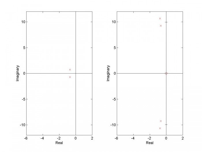
Figure B.1  s-plane transformation of N= 2 lowpass poles to bandpass poles and zeros.

                      Left:  Normalized lowpass Complex-conjugate poles, N= 2

                      Right:  Bandpass poles and zero for Ω₀= 10 rad/s and BW= 2 rad/s

                      The zero at s= 0 is 2^nd order.

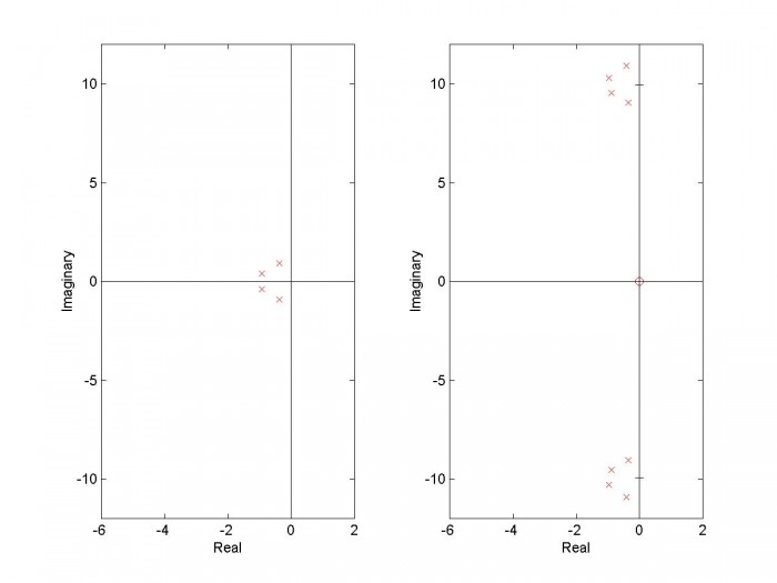
Figure B.2  s-plane transformation of N= 4 lowpass poles to bandpass poles and zeros.

                      Left:  Normalized lowpass Complex-conjugate poles, N= 4

                      Right:  Bandpass poles and zeros for Ω₀= 10 rad/s and BW= 2 rad/s

                      The zero at s= 0 is 4^th order.

Zeros of H(s) and H(z)

Consider a single-pole normalized lowpass transfer function in s’:

$$H(s')=\frac{1}{s'-\alpha}$$

It has a zero at s’= infinity.  From B-1, we have for the corresponding bandpass filter:

$$H(s)=\frac{1} {\frac{\Omega_0}{BW}\left(\frac{s}{\Omega_0}+\frac{\Omega_0}{s}\right)-\alpha}$$

H(s) has a zero at s= 0 and a zero at infinity.  In general, if H(s’) has N zeros at infinity, then H(s) has N zeros at 0 and N zeros at infinity. 

In my last post [1], I showed that the bilinear transform maps a zero at infinity to one at f_s/2.  Thus z = exp(j2πf/f_s) = exp(jπ) = -1.  For a zero at s= 0, z= exp(j0)= 1.  We can now write H(z) in pole-zero format as:

$$H(z)=K\frac{(z+1)^N(z-1)^N}{(z-p_1)(z-p_2)...(z-p_{2N})}$$

The numerator of H(z) can be written as $(z^2-1)^N$.  If you expand this, you get the numerator polynomial coefficients as follows:

     N= 1:  b= [1 0 -1]
     N= 2:  b= [1 0 -2 0 1]
     N= 3:  b= [1 0 -3 0 3 0 -1]

Thus odd-power numerator coefficients are always zero and all numerator coefficients are integers before scaling by K.

Figure B.3 shows the z-plane pole-zero plot of a bandpass filter based on a 4^th order Butterworth lowpass.  You can compare it to the pole-zero plot of the continuous-time bandpass filter in Figure B.2.

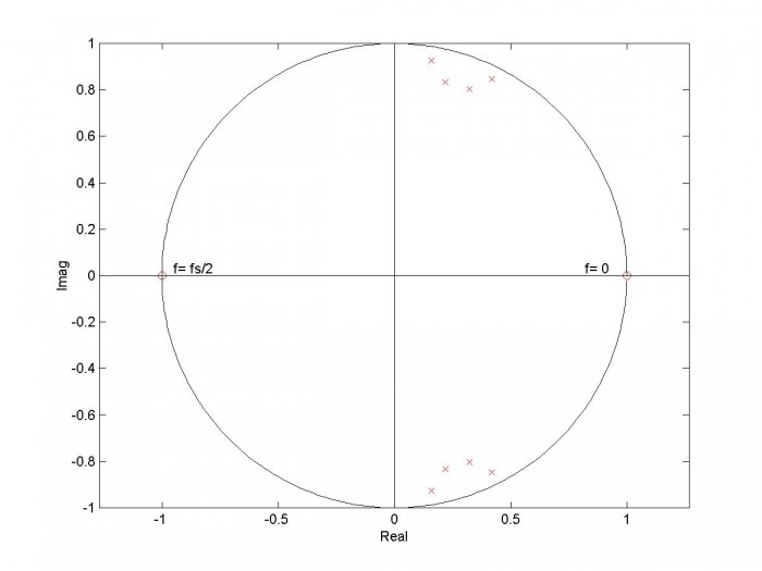
Figure B.3.  Z-plane pole-zero plot of bandpass filter based on 4^th order lowpass prototype.

                  fcenter= 20 Hz, bw= 5 Hz, and fs= 100 Hz.  Zeros at z= +/-1 are 4^th order.

Appendix C  Notation

In this article, we added to the notation used in the post on lowpass filter synthesis [1].

Notation for normalized lowpass continuous frequencies:

normalized radian frequency                    Ω’  rad/s

normalized complex frequency                 s’= σ + jΩ’

Notation for bandpass filter continuous frequencies:

-3 dB frequencies                                       Ω₁, Ω₂  rad/s

-3 dB bandwidth                                         BW  rad/s

geometric mean frequency                        $\Omega_0=\sqrt{\Omega_1\Omega_2}$   rad/s

- 3 dB bandwidth, Hz                                   BW_Hz  Hz

geometric mean frequency, Hz                   F₀  Hz

Notation for bandpass filter discrete frequencies:

-3 dB frequencies, Hz                                 f₁, f₂  Hz

geometric mean frequency, Hz                  f₀  Hz

The notation already developed in the previous post:

continuous frequency                                  F  Hz

continuous radian frequency                      Ω  radians/s

complex frequency                                      s = σ + jΩ

discrete frequency                                       f  Hz

discrete normalized radian frequency         ω = 2πf/f_sradians, where f_s = sample frequency

Finally, the Matlab function represents -3 dB discrete bandwidth (Hz) as bw and the -3 dB continuous bandwidth (Hz) as BW_hz.

References

1.  Robertson, Neil , “Design IIR Butterworth Filters Using 12 Lines of Code”, Dec 2017 https://www.dsprelated.com/showarticle/1119.php  

2.  Williams, Arthur B. and Taylor, Fred J., Electronic Filter Design Handbook, 3^rd Ed., McGraw-Hill, 1995, section 2.3

3.  Analog Devices Mini Tutorial MT-224, 2012 http://www.analog.com/media/en/training-seminars/tutorials/MT-224.pdf

4.  Oppenheim, Alan V. and Shafer, Ronald W., Discrete-Time Signal Processing, Prentice Hall, 1989, sections 6.8 and 6.9.

5.   Lyons, Richard G., Understanding Digital Signal Processing, 2^nd Ed., Pearson, 2004, section 6.7

6.  Blinchikoff, Herman J., and Zverev,Anatol I., Filtering in the Time and Frequency Domains, Wiley, 1976, section 4.4.

7.  Nagendra Krishnapura , “E4215: Analog Filter Synthesis and Design Frequency Transformation”,  4 Mar. 2003  http://www.ee.iitm.ac.in/~nagendra/E4215/2003/handouts/freq_transformation.pdf

8.  Oppenheim, Alan V. and Shafer, Ronald W., Discrete-Time Signal Processing, Prentice Hall, 1989, section 7.2

Neil Robertson                  January, 2018        revised 4/3/2019

Sign in