Evaluate Window Functions for the Discrete Fourier Transform

The Discrete Fourier Transform (DFT) operates on a finite length time sequence to compute its spectrum.  For a continuous signal like a sinewave, you need to capture a segment of the signal in order to perform the DFT.  Usually, you also need to apply a window function to the captured signal before taking the DFT [1 - 3].  There are many different window functions and each produces a different approximation of the spectrum.  In this post, we’ll present Matlab code that plots the spectra of windowed sinewaves for any window function, and computes figures of merit for the window function.

Background

The DFT is good at finding the spectrum of finite-duration signals, but a snag arises for signals that are continuously present over long duration, for example, a sinewave.  The snag is apparent in the DFT formula, which is defined over a finite number of samples N:

$$X(k)=\sum_{n=0}^{N-1}x(n)e^{-j2\pi kn/N} $$

Where

X(k) = discrete frequency spectrum of time sequence x(n)

n = time index

k = frequency index

N = number of samples of x(n) and X(k)

So, by its definition, the DFT does not apply to infinite duration signals.

Figure one is an example of a finite-duration signal – it is fully captured in less than 256 time samples.  On the other hand, the sinewave at the top of Figure 2 has an infinite number of samples.  If we try, as in the bottom of Figure 2, to capture a chunk of it and take the DFT, there is no reason to expect a happy result.  The mismatch in amplitude between the two ends of the signal distorts the spectrum, a phenomenon called spectral leakage.  We would have to capture an exact integer number of periods to get an accurate spectrum.

The way around this problem is illustrated in Figure 3.  In this example, we capture 128 samples of the sinewave, then multiply each sample by the corresponding sample of the window function shown in the middle plot, which has the property of smoothly approaching zero at each end.  The result is the “windowed” sinewave at the bottom, which is now a finite-duration signal.  This more or less works, but as we’ll see, the spectrum is that of the captured signal convolved with the spectrum of the window.  Next, we’ll look at the spectrum of a window and then apply the window to a sinewave.

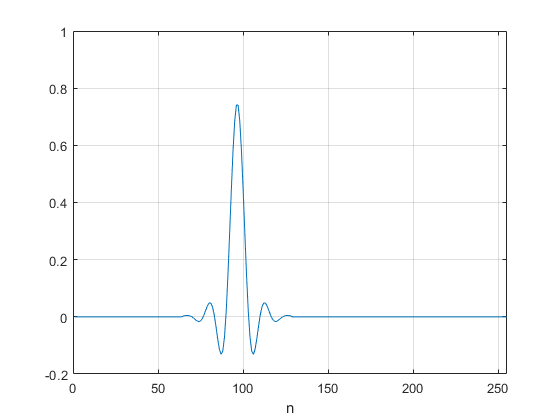
Figure 1.  Signal of finite duration                                 

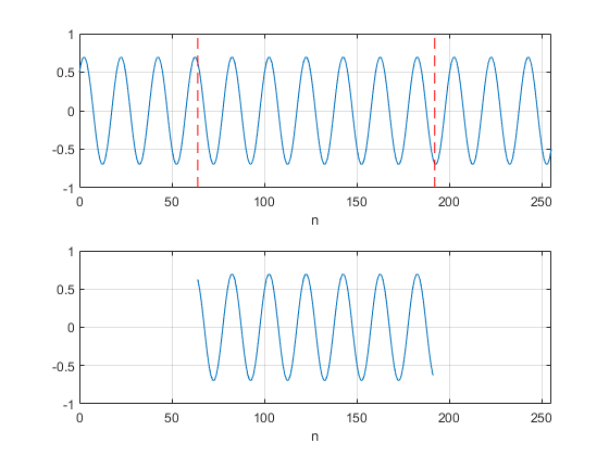
Figure 2.  Top:  Signal of infinite duration.  Bottom:  128-point capture of signal.         

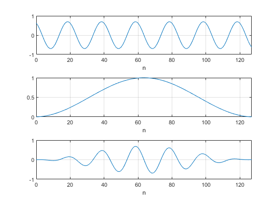
Figure 3.  Top:  Captured sinewave                          

Middle:  Window function        

Bottom:  Windowed sinewave

Spectrum of the Hanning Window

One commonly used window, the Hann, or Hanning window, is defined by this formula [4]:

$$w(n)=0.5(1-cos(2\pi n/N)), \quad n=0:N-1$$

As an example, for N = 8, we have:  w = [0  0.1464  0.5  0.8536  1  0.8536  0.5  0.1464].  We can create an N= 32 Hanning window as follows:

     N= 32;                            % number of time samples
     win= hanning(N,'periodic');        % hanning window

The window is plotted at the top of figure 4.  Now we’ll look at the spectrum of the window.  We can approximate the Fourier Transform of the window by appending zeros to the window (zero-padding) and taking the DFT.  If we zero-pad such that the number of samples is increased by a factor of L, then the DFT frequency spacing is reduced by a factor of L compared to the N-point DFT [5].  For large enough L, all the important detail of the Fourier Transform is displayed by the DFT.  The Matlab fft function fft(x,NFFT) automatically appends zeros to x to length NFFT.  Here is the code to find the spectrum of the hanning window:

     win= win/sum(win);                    % scale window for |h(0)| = 1
     % NFFT-point FFT of N-point window function
     fs= 16;                               % Hz sample frequency
     L= 32;
     NFFT= L*N;
     k= 0:NFFT/2-1;                        % freq index for NFFT-point FFT
     f= k*fs/NFFT;                         % Hz frequency vector
     h = fft(win,NFFT);                    % FFT of length NFFT (zero padded)
     h= h(1:NFFT/2);                       % retain points from 0 to fs/2
     HdB= 20*log10(abs(h));                % dB magnitude of fft

The dB-magnitude spectrum is plotted in the bottom plot of Figure 4.  

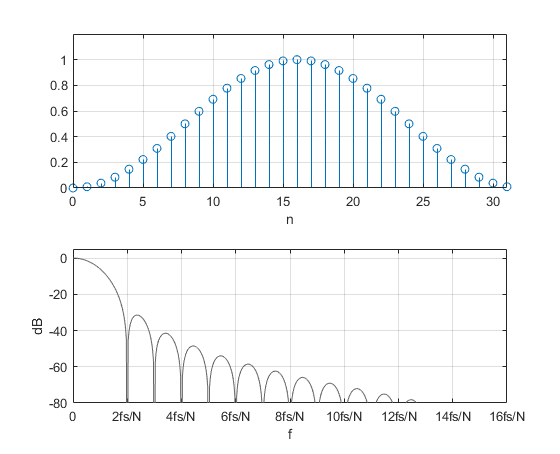
Figure 4. Top:  Hanning window, N= 32        

   Bottom:  Spectrum of Hanning window for FFT length = N*32        

Windowing a Sinewave

Now we’ll look at the spectrum of windowed sinewaves.  It will behoove us to keep careful track of the power of the signal and its spectrum.

First, we define the window, then scale it such that the power of the window function is 1 watt (refer to my earlier post on the power spectrum [6]).  

     fs= 16;                           % Hz sample frequency
     N= 32;                            % number of time samples
     win= hanning(N,'periodic');       % hanning window
     win= win.*sqrt(N/sum(win.^2));    % normalize window for P = 1 W

Now define the sinewave.  In this example, we let the sine frequency f₀ = 4*f_s/N = 4*16/32= 2 Hz.  This sinewave has exactly 4 of periods over N, and f₀ falls exactly on a DFT frequency sample – i.e. the center of a DFT bin.

    A= sqrt(2);                    % sine amplitude for P= 1 W
    Ts= 1/fs;
    n= 0:N-1;                      % s time index
    f0 = 4*fs/N;                   % Hz f0= 2 Hz
    x= A*sin(2*pi*f0*n*Ts);        % sine at bin center, P= 1 watt

Next apply the window and find the DFT by using the Matlab fft function.  The Matlab operator .* indicates element-by-element multiplication, or dot product.  The prime on win’ creates a row vector from the column vector win.  We compute both the N*L-point and N-point DFT, and scale to obtain power into a one-ohm load.

    xw= x.*win';                 % apply window to sinewave
    X= fft(xw,NFFT);             % FFT of length NFFT (zero padded)
    X= X(1:NFFT/2);              % retain points from 0 to fs/2
    P= 2/N.^2 * abs(X).^2;       % power spectrum into 1 ohm
    PdB= 10*log10(P);            % dB magnitude of zero-padded FFT
    PdB_dec= PdB(1:L:NFFT/2);    % dB magnitude of non zero-padded FFT

The N-point and N*L-point DFT’s are plotted in the top of Figure 5.  Each spectrum is just that of the Hanning window in Figure 4 convolved with that of a sinewave at 2 Hz (multiplication in the time domain is equivalent to convolution in the frequency domain).  Unlike the ideal sine spectrum, the windowed spectrum has a finite bandwidth and sidelobes.  The -40 dB bandwidth of the main lobe is about 4f_s/N = 4*16/32 = 2 Hz.  The bandwidth is inversely proportional to the number of samples N of the captured sinewave.

For an unwindowed sine at bin center, we expect the spectral peak to be 0 dB (1 watt into 1 ohm).  But the peak of the spectrum using the Hanning window is -1.74 dB because the power is spread over several samples instead of all being contained in one sample.  If power of a narrowband spectral component is important, this reduction of the peak level, called processing loss, should be taken into account.

Processing loss is proportional to the bandwidth of the window.  In fact, it is exactly equal to the noise bandwidth (in bins) of the window (see appendix B).  As a practical matter, higher processing loss/noise bandwidth makes it harder to discern a low-level signal in the presence of noise (it gets hidden by the noise floor) and degrades the ability to resolve signals that are closely-spaced in frequency.

Now let f₀ = 4.5 f_s/N.  This sinewave has 4.5 periods over N, and f₀ falls exactly between DFT frequency samples – i.e. the edge of a DFT bin.

    f0 = 4.5*fs/N;                % Hz f0= 2.5 Hz
    x= A*sin(2*pi*f0*n*Ts);       % sine at bin edge, P= 1 watt

If we window this sinewave and find the DFT’s as above, we get the spectra plotted in the bottom of Figure 5.  The N*L-point DFT has the same shape as the spectrum at bin center.  However, the N-point DFT has a different peak value and higher skirts.  The difference in peak value is about 1.44 dB for the Hanning window.  So here is another source of error in the displayed spectrum.  This variation in the DFT amplitude is called scalloping loss [7].  Note that scalloping is only an issue for narrowband signals that have bandwidth less than the frequency bin of the DFT.

To summarize, here is a list of properties of a sinewave’s windowed spectrum:

• There is a main lobe with bandwidth proportional to 1/N.
• There are typically sidelobes with finite attenuation.
• For a sine at bin center, processing loss is the level of the spectral peak relative to that of an unwindowed sine.
• The noise bandwidth in bins is equal to the processing loss (Appendix B).
• Depending on the window used, scalloping loss occurs when the sine frequency is not at the center of a bin.

The 3-dB or 6-dB bandwidth of the main lobe is sometimes called resolution bandwidth.  The sidelobe level with respect to the main lobe peak level is sometimes called dynamic range.  Dynamic range is a measure of the ability to discern a small signal in the presence of a larger signal.  Note that for the Hanning window, the sidelobes of the N-point DFT’s (blue curves of Figure 5) are not visible as distinct features.

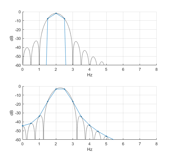
Figure 5.  Top:  Spectrum of Windowed Sine with f₀ = 4*fs/N = 2 Hz (center of bin)

Bottom:  Spectrum of Windowed Sine with f₀ = 4.5*fs/N = 2.5 Hz (edge of bin)

A Matlab Function to Evaluate Windows

The Matlab function win_plot(win,fs) is listed in Appendix A.  This function computes several window figures of merit, and plots the windowed N-point DFT of two sine waves located at f₀= f_s/8 (center of a bin) and f₁= f_s/4 + .5f_s/N (edge of a bin), where N is the length of the window win.  The inputs to the function are a window vector win and sample frequency fs (Hz).  The length of win must be a power of 2.

If f_s is set equal to length(win), then frequency is equal to bin number and the x-axis units are indicated as “bins”.

Here is an example using the Hanning window of length 256 and f_s= 200 Hz.  The function outputs the figures of merit shown and plots the DFT spectrum.

    win= hanning(256,'periodic');
    win_plot(win,200)
        noise bw (bins)  1.4942
        proc loss (dB)  1.744
        max proc loss (dB)  3.1789
        scallop loss (dB)  1.435

As shown in Figure 6, The output spectrum is plotted twice, with two different amplitude scales.  The top plot has a 10 dB range and the bottom plot has a 120 dB range.  The lower frequency sine at a bin center shows the processing loss of 1.74 dB.  The upper frequency sine at a bin edge shows the max processing loss of 3.18 dB.  Scallop loss is the difference of these two values.

If we want the x-axis units in bins, we set fs = length(win) = 256:

    win= hanning(256,'periodic');
    win_plot(win,256)

The resulting plot is shown in Figure 7, which is identical to figure 6, except that the x axis is in bins instead of Hz.  Like the blue curves in Figure 5, the sidelobes are not individually visible for this N-point FFT.  The spectrum of the sinewave located at a bin edge is about -50 dB at 5 bins from the center.

In summary, the Hanning window has low processing loss/noise bandwidth, but only modest dynamic range.

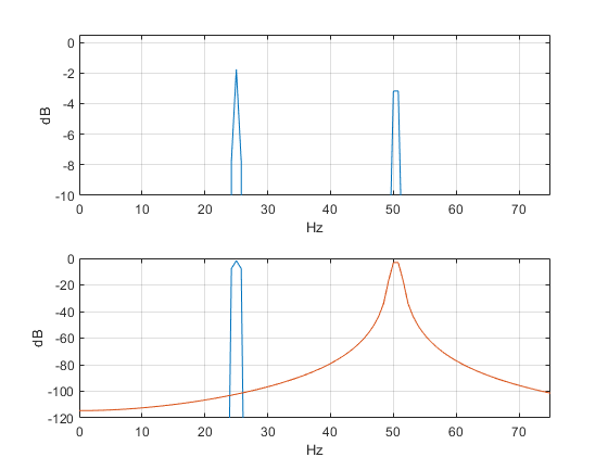
Figure 6.  Output spectra of win_plot(win,200) for win = hanning(256,'periodic')

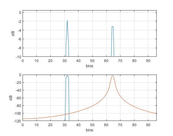
Figure 7.  Output spectra of win_plot(win,256) for win = hanning(256,'periodic')

f_s = 256 = length(win), causing x-axis units to be bins

Processing loss = 1.74 dB; noise bw = 1.5 bins; scallop loss = 1.44 dB

Window Examples using win_plot

Now let’s look at a few more windows.  See Table 1 for a comparison of their figures of merit.

1. No Window

    win= rectwin(256);
    win_plot(win,256);

Having no window is equivalent to a window that is all ones – the rectangular (boxcar) window of Figure 8.  Figure 9 shows the spectrum. Processing loss is ideal at 0 dB, but spectral leakage is massive for the sinewave at the edge of a bin.

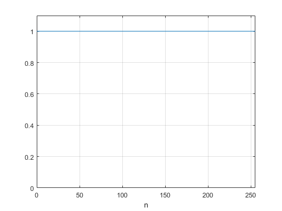
Figure 8.Rectangular or boxcar window, N= 256              

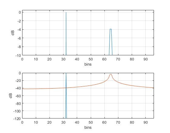
Figure 9.  Output spectra of win_plot(win,256) for win = rectwin(256)         

Processing loss = 0 dB; noise bw = 1 bin; scallop loss = 3.9 dB         

2. A window with no scalloping loss – flattop window

    win= flattopwin(256,'periodic');
    win_plot(win,256);

The flattop window (Figure 10) has 0 dB scalloping loss, which allows you to display the amplitude of a narrowband signal accurately, even if it falls at a bin edge.  It also has good dynamic range.  However, the processing loss/noise bandwidth are high (Figure 11).  The formula for the flattop window of length N is [8]:

$$w(n)=a_0-a_1cos\left(\frac{2\pi n}{N-1}\right) +  a_2cos\left(\frac{4\pi n}{N-1}\right)  -a_3cos\left(\frac{6\pi n}{N-1}\right)  +a_4cos\left(\frac{8\pi n}{N-1}\right), \quad n=0:N-1$$

where

a₀ = 0.21557895

a₁= 0.41663158

a₂= 0.277263158

a₃= .083578947

a₄= .006947368

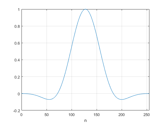
Figure 10.  Flattop Window, N= 256             

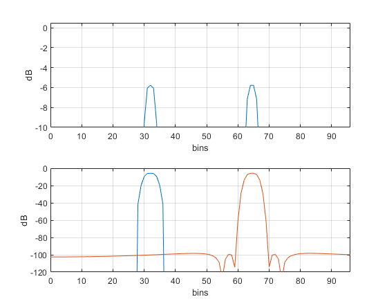
Figure 11.  Output spectra of win_plot(win,256) for win = flattopwin(256,'periodic')          

processing loss = 5.78 dB; noise bw = 3.8 bins; scallop loss = 0 dB          

3. A window with adjustable sidelobe level – Chebyshev Window

    win= chebwin(256,80);     % window with -80 dB sidelobes
    win_plot(win,256);

The Chebyshev window has flat (equiripple) sidelobes that can be adjusted to any level.  It allows you to trade bandwidth vs. sidelobe level.  Figure 12 shows the window for -80 dB sidelobes.  The spectra are shown in Figure 13.  Calculating the window function is somewhat involved; see [9,10].

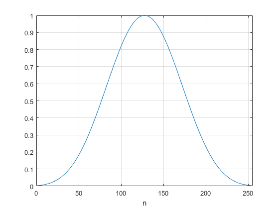
Figure 12.  -80 dB Chebyshev Window, N= 256          

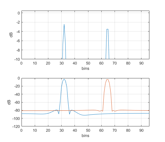
Figure 13.  Output spectra of win_plot(win,256) for win = chebwin(256,80)          

Processing loss = 2.42 dB; noise bw = 1.75 bins; scallop loss = 1.08 dB       

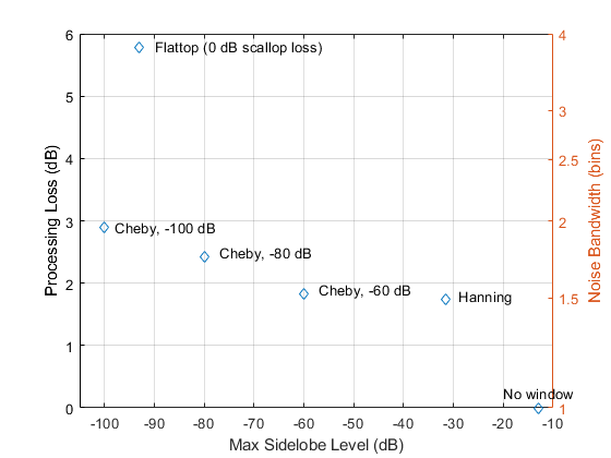
Table 1 lists figures of merit for various windows.  Figure 14 compares several window functions by plotting processing loss/noise bandwidth vs. maximum sidelobe level.  Performance increases as you move towards the lower left corner.

Table 1.Windows Figures of Merit

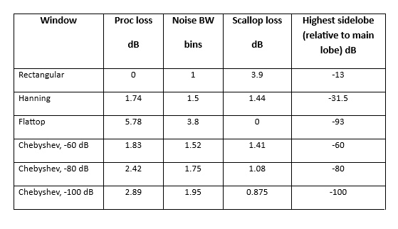
Figure 14.  Processing Loss/Noise Bandwidth vs. Maximum Sidelobe Level for various window functions.

Appendix A   Matlab Function win_plot

Calculation of the power of the DFT spectrum was discussed in an earlier post [6].

% win_plot(win,fs).m   12/13/18 Neil Robertson
%
% Evaluate window functions using sine at center of bin
% and sine at edge of bin.
%
% win  window vector, length must be a power of 2.
% fs   sample frequency in Hz
%
% ex:
% win= hanning(256);
% win_plot(win,200);
%
% Note: if fs = N = length(win), display x-axis units as "bins"
%
function win_plot(win,fs)
A= sqrt(2);                    % sine amplitude for P= 1 W
Ts= 1/fs;                      % s sample time
N= length(win);
s= size(win);
if s(2)== 1
    win= win';                 % if win is a column vector, take transpose
end
xunit= 'Hz';                   % units of plot x-axis
if fs== N
    xunit= 'bins';
    disp('fs = N: x-axis units are bins')
    disp(' ')
end
win= win.*sqrt(N/sum(win.^2));         % normalize window for P = 1
n= 0:N-1;
f0= fs/8;                              % center of bin
f1= fs/4 + .5*fs/N;                    % edge of bin
x1= A*sin(2*pi*f0*n*Ts);                % sine at center of a bin, P = 1 watt
x2= A*sin(2*pi*f1*n*Ts);                % sine at edge of a bin, P = 1 watt
% FFT of sine at bin center x1
xw= x1.*win;                            % apply window
X= fft(xw,N);
X= X(1:N/2);                            % retain samples from 0 to fs/2
P= 2/N.^2 * abs(X).^2;                  % W/bin power spectrum into 1 ohm
Pmax= max(P);                           % W/bin max of power spectrum
PdB1= 10*log10(P);
noise_bw_bins= 1/Pmax;                  % bins noise bandwidth of window
proc_loss_dB= -max(PdB1);               % dB process loss of window
% FFT of sine at bin edge x2
xw= x2.*win;
X= fft(xw,N);
X= X(1:N/2);
P= 2/N.^2 * abs(X).^2;
PdB2= 10*log10(P);
max_proc_loss_dB= -max(PdB2);                       % dB max process loss of window
scallop_loss_dB= max_proc_loss_dB - proc_loss_dB;    % dB scallop loss
% outputs
disp(['noise bw (bins)',num2str(noise_bw_bins)])
disp(['proc loss (dB)',num2str(proc_loss_dB)])
disp(['max proc loss (dB)',num2str(max_proc_loss_dB)])
disp(['scallop loss (dB)',num2str(scallop_loss_dB)])
k= 0:N/2-1;                                        % frequency index
f= k*fs/N;                                         % Hz frequency
subplot(211),plot(f,PdB1,f,PdB2,'color',[0 .447 .741]),grid
axis([0 3*fs/8 -10 .5])
xlabel(xunit),ylabel('dB')
subplot(212),plot(f,PdB1,f,PdB2),grid
axis([0 3*fs/8 -120 0])
xlabel(xunit),ylabel('dB')
subplot(111)

.

Appendix B   Noise Bandwidth

Suppose gaussian noise of density N₀ W/bin is applied to a lowpass or bandpass filter with response H(k).  Let the output noise power of the filter be P_noise.  Now, consider an ideal lowpass or bandpass filter whose output noise power for the same gaussian noise input is also P_noise.  We define the noise bandwidth of H(k) as the bandwidth of this ideal filter [11].  We also require that the maximum values of |H(k)| and the ideal filter response be the same.

Figure B.1 shows a response H(k) that happens to be that of a sinewave windowed by a flattop window (blue curve).  Also shown is an ideal filter that defines the noise bandwidth of this response.  Let P(k) be the noise power per bin into 1 ohm at the output of H(k) [6]:

$$P(k)= \frac{2}{N^2}N_0|H(k)|^2  \quad W/bin \qquad (B.1)$$

Then, from the above definition of noise bandwidth,

$$N_0*|H_{max}|^2*noise \,bandwidth=N_0* \frac{2}{N^2}\sum_{k=0}^{N/2-1}|H(k)|^2 \qquad (B.2)$$

Where

N₀ = Input noise density, W/bin

|H_max|= maximum value of |H(k)| (dimensionless)

Noise bandwidth = bins

N = number of samples in two-sided response

Noise bandwidth is then

$$ noise \,bandwidth= \frac{1}{|H_{max}|^2}\frac{2}{N^2}\sum_{k=0}^{N/2-1}|H(k)|^2 \quad bins \qquad (B.3)$$

For a normalized window function [6], the numerator term is 1, and we have simply

$$noise \,bandwidth \quad(bins)=\frac{1}{|H_{max}|^2} \qquad (B.4) $$

For a windowed sinewave, |H_max|² is just 1/processing loss.  (For a normalized window function, |H_max|² < 1).  For example, processing loss of the Flattop window spectrum of Figure B.1 is 5.781 dB.  This is a magnitude of 10^(5.781/10) = 3.78.  Thus, noise bandwidth is 3.78 bins.

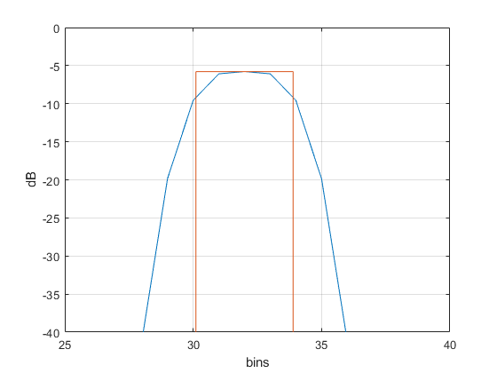
Figure B.1  A frequency response (blue curve) and the ideal response defining its noise bandwidth.

.

References

1. Lyons, Richard, “Widowing Functions Improve FFT Results”, EDN, June 1, 1998.  https://www.edn.com/electronics-news/4383713/Windowing-Functions-Improve-FFT-Results-Part-I    
2.  Rapuano, Sergio, and Harris, Fred J., An Introduction to FFT and Time Domain Windows, IEEE Instrumentation and Measurement Magazine, December, 2007. https://ieeexplore.ieee.org/document/4428580
3.  Harris, Fredric J., “On the Use of Windows for Harmonic Analysis with the Discrete Fourier Transform”, Proc. IEEE, vol 66, pp. 51-83, Jan 1978. https://www.utdallas.edu/~cpb021000/EE%204361/Great%20DSP%20Papers/Harris%20on%20Windows.pdf 
4.   Lyons, Richard, Understanding Digital Signal Processing , Third Ed., Prentice Hall, 2011, p 91.
5. Lyons, section 3.11.
6. Robertson, Neil, “The Power Spectrum” https://www.dsprelated.com/showarticle/1004.php
7. Lyons, section 3.10
8. Mathworks website https://www.mathworks.com/help/signal/ref/flattopwin.html
9. Lyons, Richard, “Computing Chebyshev Window Sequences” https://www.dsprelated.com/showarticle/42.php
10. Wikipedia https://en.wikipedia.org/wiki/Window_function#Dolph%E2%80%93Chebyshev_window
11. Harris, Op. cit.

Neil Robertson    December, 2018       Revised 2/22/20, 11/20/21, 3/23/23

Sign in