


IIR Bandpass Filters Using Cascaded Biquads
In an earlier post [1], we implemented lowpass IIR filters using a cascade of second-order IIR filters, or biquads.
This post provides a Matlab function to do the same for Butterworth bandpass IIR filters. Compared to conventional implementations, bandpass filters based on biquads are less sensitive to coefficient quantization [2]. This becomes important when designing narrowband filters.
A biquad section block diagram using the Direct Form II structure [3,4] is shown in Figure 1. It is defined by two feedback coefficients a, three feed-forward coefficients b, and gain K. There can be one or more cascaded biquad sections in a bandpass filter. The function biquad_bp (listed in the Appendix) computes biquad coefficients and gains given the order of the lowpass prototype, center frequency, bandwidth, and sampling frequency. For a lowpass prototype of order N, the bandpass filter has order 2N and requires N biquads.
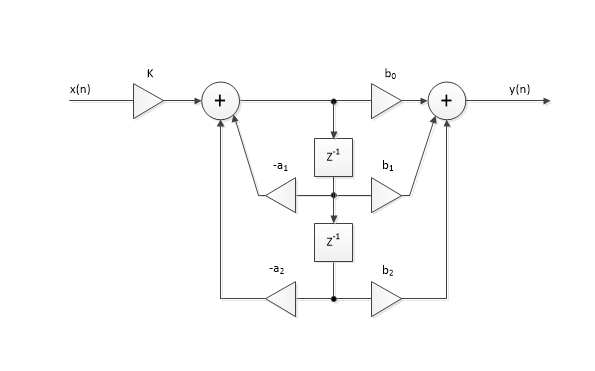
Figure 1. Biquad Section Block Diagram.
Example 1.
Here is an example function call and results for a bandpass filter based on a 3rd order lowpass prototype:
    N= 3;               % order of prototype LPF (number of biquads in BPF)
    fcenter= 20;        % Hz center frequency
    bw= 4;              % Hz -3 dB bandwidth
    fs= 100;            % Hz sample frequency
    [a,K]= biquad_bp(N,fcenter,bw,fs)
        a = 1.0000  -0.3835  0.8786
            1.0000  -0.5531  0.7757
            1.0000  -0.7761  0.8865
                                                                 .
        K = 0.1254  0.1122  0.1114
The function generates N = 3 sets of biquad feedback coefficients in the matrix a, plus a gain K for each biquad section. The gains K are computed to make the response magnitude of each section equal 1.0 at approximately fcenter. We can use a and K to find the frequency response of the biquads. As we’ll show later, the feed-forward coefficients of the biquads are all the same: b = [1 0 -1]. We assign the parameters of each biquad as follows:
    b= [1 0 -1];            % feed-forward coeffs of each biquad
    a_bq1= a(1,:);          % biquad 1 feedback coeffs = [1 -.3835 .8786]
    a_bq2= a(2,:);          % biquad 2 feedback coeffs = [1 -.5531 .7757]
    a_bq3= a(3,:);          % biquad 3 feedback coeffs = [1 -.7761 .8865]
    K1= K(1); K2= K(2); K3= K(3);    % biquad gains
Now we can compute the frequency response of each biquad.
    [h1,f]= freqz(K1*b,a_bq1,2048,fs);    % frequency response
    [h2,f]= freqz(K2*b,a_bq2,2048,fs);
    [h3,f]= freqz(K3*b,a_bq3,2048,fs);
    H1= 20*log10(abs(h1));                % dB-magnitude response
    H2= 20*log10(abs(h2));
    H3= 20*log10(abs(h3));
These responses are plotted in Figure 2. Computing the response of the cascaded biquads:
    h= h1.*h2.*h3;
    H= 20*log10(abs(h));
This overall response is shown in Figure 3. Given feed-forward coefficients b= [1 0 -1], the block diagram of each biquad is as shown in Figure 4. The coefficient a0 = 1.0 is not used. Note that the feedback gains have negative signs, so given a1 = -.3835 and a2= .8786, the feedback gains are .3835 and -.8786.
Looking at Figure 2 again, note that the first and last biquads have response magnitude that is greater than 1.0 (0 dB) at some frequencies, even though the response is 0 dB near fcenter = 20 Hz. When implementing a fixed-point filter, we need to take this into account to avoid overflow. For this example, overflow is most likely if the input has a large component at the peak of the response of the first biquad, which occurs at about 22 Hz. To prevent overflow, we could allow extra headroom in the first biquad; swap the 2nd biquad with the first biquad; or reduce the gain K1 while maintaining the product of the biquad gains constant.
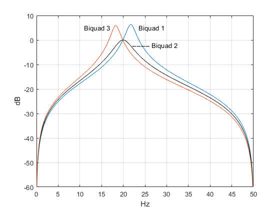
Figure 2. Response of each biquad section for N= 3, center frequency = 20 Hz,
bandwidth = 4 Hz, and fs= 100 Hz.
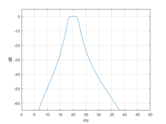
Figure 3. Overall response of bandpass filter.
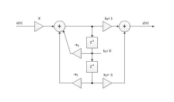
Figure 4. Biquad section for a bandpass filter.
How biquad_bp Works
In an earlier post on IIR bandpass filters [5], I presented the pole-zero form of the bandpass response as:
$$
H(z)=K\frac{(z+1)^N(z-1)^N}{(z-p_1)(z-p_2)...(z-p_{2N})}\qquad(1)$$
where N is the order of the prototype lowpass filter. Calculation of the pk was described in the post. For a bandpass filter, the 2N poles occur as complex-conjugate pairs. For example, the poles of the filter of Example 1 are shown in Figure 5. There are also N zeros at z= -1 and N zeros at z= +1. Our goal is to convert H(z) into a cascade of second-order sections (biquads). We can do this by writing H(z) as the product of N sections with complex-conjugate poles:
Where p*k is the complex conjugate of pk. Note we have assigned a zero at z= -1 and a zero at z = +1 to each biquad. We could assign the zeros differently, but this method is straightforward and gives reasonable results. Expanding the numerator and denominator of the kth biquad section, we get:
$$ H_k(z)=K_k\frac{z^2-1}{z^2-(p_k+p_k^*)z+p_kp_k^*}$$
$$ =K_k\frac{z^2-1}{z^2+a_1z+a_2}$$
where a1= -2*real(pk) and a2= |pk|2. Dividing numerator and denominator by z2, we get:
$$
H_k(z)=K_k\frac{1-z^{-2}}{1+a_1z^{-1}+a_2z^{-2}}\qquad(3)$$
Since we assigned the same zeros to each biquad, the numerator (feed-forward) coefficients b = [1 0 -1] are the same for all N biquads. Summarizing the biquad coefficient values, we have:
b = [1 0 -1]
a = [1 -2*real(pk) |pk|2] (4)
To find the gains Kk, we let each biquad have gain of 1 at the filter geometric mean frequency f0. We do this by evaluating Hk(z) at f0 and setting Kk = 1/|H(f0)|. To find f0, we define f1= fcenter – bw/2 and f2= fcenter+bw/2. Then $f_0=\sqrt{f_1*f_2} $. Note that for a narrowband filter, f0 is close to fcenter.
The Matlab code to find Kk is:
    f0= sqrt(f1*f2);
    h= freqz(b,a,[f0 f0],fs);     % frequency response at f = f0
    K= 1/abs(h(1));
The biquad section with coefficients b, a, and gain K is shown in Figure 4. Here is a summary of the filter synthesis steps used by biquad_bp (The first four steps are detailed in [5]):
- Find the poles of a lowpass analog prototype filter with Ωc = 1 rad/s.
- Given upper and lower -3 dB frequencies of the digital bandpass filter, find the corresponding frequencies of the analog bandpass filter (pre-warping).
- Transform the analog lowpass poles to analog bandpass poles.
- Transform the poles from the s-plane to the z-plane, using the bilinear transform.
- Compute the feedback (denominator) coefficients of each biquad using Equation 4 above.
- Compute the gain K of each biquad.
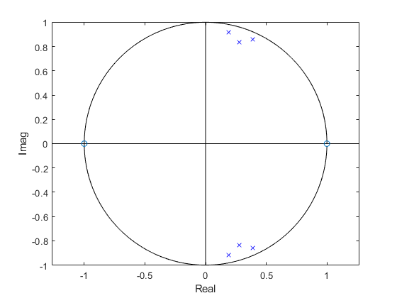
Figure 5. Z-plane poles and zeros of the bandpass filter of Example 1.
Example 2 – Narrow bandpass filter with quantized coefficients
Let’s try implementing a narrow band-pass filter with quantized denominator coefficients. We’ll use a bandwidth of 0.5 Hz with sampling frequency of 100 Hz. With lowpass prototype of 3rd order and center frequency of 22 Hz, the function call and results are:
N= 3;                % order of prototype LPF
fcenter= 22;         % Hz center frequency
bw= .5;              % Hz -3 dB bandwidth
fs= 100;             % Hz sample frequency
[a,K]= biquad_bp(N,fcenter,bw,fs)
    a = 1.0000  -0.3453  0.9844
        1.0000  -0.3690  0.9691
        1.0000  -0.3983  0.9845
                                                         .
    K = 0.0157  0.0155  0.0155
Now assign the numerator coefficients and quantize the
denominator coefficients to 12 bits:
    b= [1 0 -1];                        % numerator coeffs
    nbits= 12;                          % bits per unit amplitude
    a_quant= round(a*2^nbits)/2^nbits;  % quantize denominator coeffs
Computing the frequency response as was done in Example 1, we get the response shown in Figure 6. Figure 7 shows the response at 1 dB per division for 12-bit and 8-bit denominator coefficients. As you can see, we get good results using 12-bit coefficients, and some response degradation using 8-bit coefficients. Figure 8 shows three of the six poles of the filter, which are very close to the unit circle compared to the less narrow filter of Example 1 (Figure 5). A conventional bandpass implementation with quantized coefficients could easily become unstable due to the poles falling outside the unit circle.
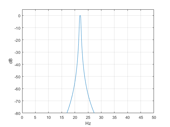
Figure 6. Response of bandpass with N = 3, bw = 0.5 Hz, and denominator coefficients = 12 bits.
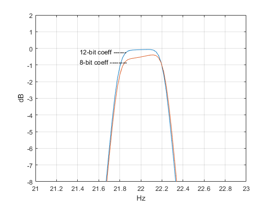
Figure 7. Bandpass filter response vs. denominator coefficient quantization.
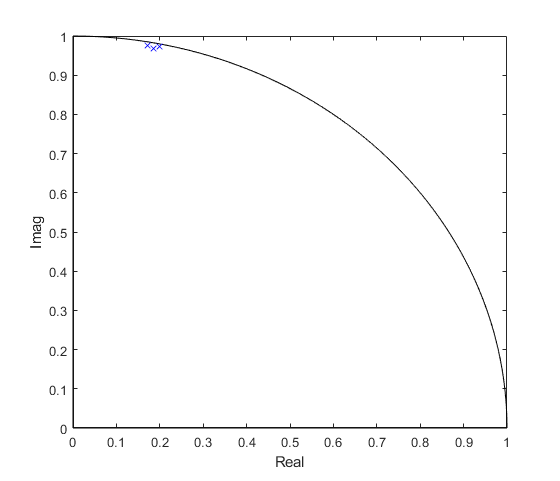
Figure 8. Three of six z-plane poles of the filter of Example 2.
Appendix Matlab Function biquad_bp
Some of the formulas in this program were developed in an earlier post on bandpass IIR filters [5]. This program is provided as-is without any guarantees or warranty. The author is not responsible for any damage or losses of any kind caused by the use or misuse of the program.
Note: This program assumes the poles of the filter transfer function are complex-conjugate. However, when the lowpass prototype order N is odd and bw is large compared to fcenter, there can be real poles. When N is odd, the results will be incorrect if BW_hz > 2*F0 (see the code for definitions of these parameters).
%function [b,a]= biquad_bp(N,fcenter,bw,fs)  4/7/19  Neil Robertson
% Synthesize IIR Butterworth Bandpass Filters using biquads
%
% N= order of prototype LPF = number of biquads in BPF
% fcenter= center frequency, Hz
% bw= -3 dB bandwidth, Hz
% fs= sample frequency, Hz
% a= matrix of denominator coefficients of biquads.
%    each row contains the denom coeffs of a biquad.
%    There are N rows.
% K= vector of gain blocks for each biquad.Length = N.
%
% Note:numerator coeffs of each biquad = K(k)*[1 0 -1]
%
function [a,K]= biquad_bp(N,fcenter,bw,fs)
f1= fcenter- bw/2;                % Hz lower -3 dB frequency
f2= fcenter+ bw/2;                % Hz upper -3 dB frequency
if f2>=fs/2;
    error('fcenter+ bw/2 must be less than fs/2')
end
if f1<=0
    error('fcenter- bw/2 must be greater than 0')
end
% find poles of butterworth lpf with Wc = 1 rad/s
k= 1:N;
theta= (2*k -1)*pi/(2*N);
p_lp= -sin(theta) + j*cos(theta);
% pre-warp f0, f1, and f2 (uppercase == continuous frequency variables)
F1= fs/pi * tan(pi*f1/fs);
F2= fs/pi * tan(pi*f2/fs);
BW_hz= F2-F1;                % Hz -3 dB bandwidth
F0= sqrt(F1*F2);             % Hz geometric mean frequency
% transform poles for bpf centered at W0
% pa contains N poles of the total 2N -- the other N poles not computed
% are conjugates of these.
for i= 1:N;
    alpha= BW_hz/F0 * 1/2*p_lp(i);
    beta= sqrt(1- (BW_hz/F0*p_lp(i)/2).^2);
    pa(i)= 2*pi*F0*(alpha +j*beta);
end
% find poles of digital filter
p= (1 + pa/(2*fs))./(1 - pa/(2*fs));    % bilinear transform
% denominator coeffs
for k= 1:N;
    a1= -2*real(p(k));
    a2= abs(p(k))^2;
    a(k,:)= [1 a1 a2];                 % denominator coeffs of biquad k
end
b= [1 0 -1];                           % biquad numerator coeffs
% compute biquad gain K for response amplitude = 1.0 at f0
f0= sqrt(f1*f2)                        % geometric mean frequency
for k= 1:N;
    aa= a(k,:);
    h= freqz(b,aa,[f0 f0],fs);         % frequency response at f = f0
    K(k)= 1/abs(h(1));
end
References
- Robertson, Neil, “Design IIR Filters Using Cascaded Biquads”, Feb, 2018, https://www.dsprelated.com/showarticle/1137.php
- Oppenheim, Alan V. and Shafer, Ronald W., Discrete-Time Signal Processing, Prentice Hall, 1989, section 6.9.
- Sanjit K. Mitra, Digital Signal Processing, 2nd Ed., McGraw-Hill, 2001, section 6.4.1
- “Digital Biquad Filter”, https://en.wikipedia.org/wiki/Digital_biquad_filter
- Robertson, Neil, “Design IIR Bandpass Filters”, Jan, 2018,
https://www.dsprelated.com/showarticle/1128.php
April, 2019 Neil Robertson Appendix revised 5/14/2020


- Comments
- Write a Comment Select to add a comment

i remember when i was an undergrad in the 1970s taking a class in television engineering and learning how to make a sharp cutoff and flat passband filter by cascading 2nd-order BPF sections. so my question to Neil is, how might this example (Figs. 2 and 3) compare to a 6th-order Butterworth BPF (which would be mapped from a 3rd-order Butterworth LPF)? otherwise, i dunno how one chooses the Q or bw of each 2nd-order section to give you the flat response that you spec'd .
the other question i was going to ask is about the coefficient quantization. when does that come into play? in an FPGA? especially 8-bit quantization. i dunno of any modern machine that would impose such coarse quantization as that.

Hi RBJ,
I wrote a previous post on IIR BPF's synthesized directly from the LP prototype. Figure 3 shows the response of different order Butterworth bandpass filters, including a 6th order BPF based on a 3rd-order LPF. The response is the same as in Figure 3 of this post (plot scale is different).
You ask how one chooses the Q and BW of each biquad section: the answer is you don't have to. If you read the derivation in the post, there is no mention of Q or bandwidth of biquads. I calculate the biquad coefficients directly from the poles and zeros.
Regarding the quantization, the example given is just to illustrate the concept. I don't have a digital background, so I don't know what quantization is typical in different applications. Of course, bits get expensive as sample rate increases, so perhaps at 100's of MHz, you could benefit from 8 or 12 bit quantization.
regards,
Neil

I appreciate this article, because it's so fundamental and easy to understand, that it can be used for communication purposes to make people understand the most crititcal issues.
Or as an introductory receipt for a newcomer. Usually, most of this is in the brains, and thus difficult to show :-)
Concerning poles/zeros: one critical aspect is stability. This can be shown with the poles/zeros position: if the filter gets narrower and/or the relation of "sample frequency" / "center frequency of the BPF" increases, poles/zeros are getting very close to the unit circle.
If (especially because of coefficient word length) they happen to cross this line, instability occurs.
Instability could also happen if the word length during calculation is not big enough. But in this case, it's very difficult to detect, because Matlab (working with high resolution floating point math) might show a wonderful filter. But if implemented in µC/FPGA/HW, working with lower resolution fixed point or integer math, it might fail.
It could be a good idea to add a paragraph about stability and word length issues.
Nevertheless, I like the article. Thanks for putting it online.
Hi bholzmayer,
Thanks for these useful insights. I did mention stability in the post:
"Figure 8 shows three of the six poles of the filter, which are very close to the unit circle compared to the less narrow filter of Example 1 (Figure 5). A conventional bandpass implementation with quantized coefficients could easily become unstable due to the poles falling outside the unit circle."
regards,
Neil
Dear Neil,
thank you very much for your tutorials. They are very helpful and ejoyable!
While I was implementing your biquad based bandpass, I stumbled upon an error in the code of biquad_bp(…). I compared the characteristics against bp_synth(…) and butter(…) and found a small distortion. It depends on the choice of the parameters: The order has to be odd, so that the analog lowpass has a real pole, and the bandwidth has to be large compared to F0, so that BWhz/F0/2 > 1. In this case, the analog bandpass has two real poles, which are not simply complex conjugates, which is implicitly assumed in the code. bp_synth(…) calculates all poles without assuming any complex conjugate pairs and suffers, thus, not from this flaw.
Take for example N =3, fs = 1000, f1 = 0.05 fs, f2 = 0.25 fs (blue is biquad_bp(…) and green bp_synth(…)):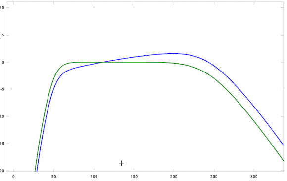
Best regards,
Andrés
Hi Andres,
Wow, this was very astute of you. Indeed, I am assuming complex-conjugate pole-pairs.
So... the limitation of biquad_bp.m is that, for N odd, BW_hz < 2*F0, where these parameters are functions of fcenter, bw, and fs. (N is the order of the LP prototype filter).
Thanks for catching this corner case.
regards,
Neil
Hi Neil,
yes, exactly. In that case the square root in the spectral transform of the BP is purely imaginary
beta= sqrt(1- (BW_hz/F0*p_lp(i)/2).^2);ending up in two real poles. Though it's a sort of corner case, it happens when large bandwidths are needed, such as in my case.
I restricted my filter to even LP orders, for which it doesn't happen, as the poles of the LP are always complex. To keep biquad_bp.m general, it would have to catch this case and treat it separately. So either the two real poles of the BP are combined into a different biquad, or two separate first order sections are used. Either of would break the nice symmetry of the code...
Best regards,
Andrés
One thing that I miss, is Biquad ordering and pole/zero pairing - this has an impact on performance.
The basic idea is that poles provide gain, and poles that are closest to the unit circle provide the highest gain. Zeros on the otherhand, provide attenuation, and can be used to 'tame' this gain. Therefore, group the poles closest to the unit circle with the zeros closest to them, and so on until all poles and zeros have been allocated. Finally, arrange the biquad cascade with the pole/zero pair closest to the unit circle (i.e. with the largest gain error) at the end of the cascade.
Here's an example for an Elliptic filter:
Regards,
Sanjeev.
Hi asn,
Thanks for this tip, which is particularly useful for filters with finite zeros. Note that for the butterworth bpf analyzed here, the zeros are all at z = -1 and z = +1. In the post, I assigned a zero at each of these locations to each biquad. I think this approach will usually work well for Butterworth bpf's.
regards,
Neil
Neil-I was wondering if you have a Mathlab Function BiQuad High Pass (HP) that you can share? I am not sure I have enough experience with the math involved to try it myself.
BTW, this BP post and the LP post are terrific. I incorporated your BP BiQuad filters in an equalizer I am building, and it is working great! The posts are very clear and easy to follow. Thanks for taking the time to put the posts together.
Neal
Neal,
The basics for a biquad HP can be summarized as follows: The LP to HP transformation of the poles is:
pa= 2*pi*Fc./p_lp;
Then the change to the numerator coeffs and scaling is:
b= [1 -2 1]; % hp biquad numerator coeffs
for i= 1:N/2;
K(i)= sum(a(i,1)- a(i,2)+ a(i,3))/4;
end
I'm glad my posts were useful to you -- thanks for the feedback.
_______________________________________________
Here is the Matlab code for biquad hp synth:
% biquad_hp.m 3/28/19 Neil Robertson
% Synthesize even-order IIR Butterworth highpass filter as % cascaded biquads.
% This function computes the denominator coeffs a of the biquads.
% N= filter order (must be even)
% fc= -3 dB frequency in Hz
% fs= sample frequency in Hz
% a = matrix of denominator coefficients of biquads.
%Size = (N/2,3)
% each row of a contains the denominator coeffs of a biquad.
% There are N/2 rows.
%
% Note numerator coeffs of each biquad= K*[1 -2 1],
%where K = (1 - a1 + a2)/4.
%
function a = biquad_synth_hp(N,fc,fs);
if fc>=fs/2;
error('fc must be less than fs/2')
end
if mod(N,2)~=0
error('N must be even')
end
% I. Find analog filter poles above the real axis
% (half of total poles)
k= 1:N/2;
theta= (2*k -1)*pi/(2*N);
p_lp= -sin(theta) + j*cos(theta); % poles of filter with
%cutoff = 1 rad/s
p_lp= fliplr(p_lp); %reverse sequence of poles – put high Q last
% II. scale poles in frequency
Fc= fs/pi * tan(pi*fc/fs); % continuous pre-warped frequency
pa= 2*pi*Fc./p_lp; % transform poles to hp
% III. Find coeffs of biquads
% poles in the z plane
p= (1 + pa/(2*fs))./(1 - pa/(2*fs)); % poles by bilinear xform
% denominator coeffs
for k= 1:N/2;
a1= -2*real(p(k));
a2= abs(p(k))^2;
a(k,:)= [1 a1 a2]; %coeffs of biquad k
end
To post reply to a comment, click on the 'reply' button attached to each comment. To post a new comment (not a reply to a comment) check out the 'Write a Comment' tab at the top of the comments.
Please login (on the right) if you already have an account on this platform.
Otherwise, please use this form to register (free) an join one of the largest online community for Electrical/Embedded/DSP/FPGA/ML engineers:


