Sum of Two Equal-Frequency Sinusoids

Some time ago I reviewed the manuscript of a book being considered by the IEEE Press publisher for possible publication. In that manuscript the author presented the following equation:

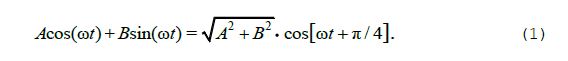
Being unfamiliar with Eq. (1), and being my paranoid self, I wondered if that equation is indeed correct. Not finding a stock trigonometric identity in my favorite math reference book to verify Eq. (1), I modeled both sides of the equation using software. Sure enough, Eq. (1) is not correct. So then I wondered, "Humm ... OK, well then just what are the correct equations for a single sinusoid equivalent of the sum of equal-frequency sine and cosine functions? This can't be too difficult." As so often happens in DSP, the answers to that simple question are much more involved than I first thought.

Why Care About The Sum of Two Sinusoidal Functions
We frequently encounter the notion of the sum of two equal-frequency (real-valued) sinusoidal functions in the literature and applications of DSP. For example, some authors discuss this topic as a prelude to introducing the concept of negative frequency [1], or in their discussions of eigenfunctions [2,3]. Also, the sum of two equal-frequency sinusoids can be used to generate information-carrying signals in many digital communications systems, as well as explain the effects of what is called multipath fading of radio signals [4].

The Sum of Two Real-Valued Sinusoidal Functions
As you might expect, the sum of two equal-frequency real sinusoids is itself a single real sinusoid. However, the exact equations for all the various forms of that single equivalent sinusoid are difficult to find in the signal processing literature. Here we provide those equations:

• Table 1 gives the sum of two arbitrary cosine functions.
• Table 2 gives the sum of two arbitrary sine functions.
• Table 3 gives the sum of an arbitrary cosine and an arbitrary sine function.

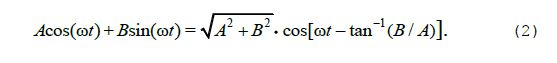
In those tables, variables A and B are real-valued scalar constants, frequency ω is in radians/second, and variables α and β are phase angles measured in radians. The various forms of the sum of two real sinusoids are in the leftmost table columns. The single-sinusoid equivalents are in the rightmost columns. (Their derivations are provided at the end of this material.) As an example, the sixth row of Table 3 tells us that the correct form for the above incorrect Eq. (1) is:

NOTE: Several months after I created the equations in the above tables I ran across somewhat similar material on the Internet written by the prolific Julius O. Smith III. In that material Prof. Smith presents equations for the general case of summing N ≥ 2 arbitrary cosine functions of the same frequency. That material can be found at the web page given in Reference [2].

Derivation Methods
Deriving the closed-form expressions for the sum of two equal-frequency sinusoidal functions is most easily accomplished by first finding the expression for the sum of two arbitrary equal-frequency complex exponentials. So that's where I started.

The Sum of Two Complex Exponentials
First we identify a general complex exponential as:

where the left-side exponential's magnitude is the constant scalar A. Frequency ω is in radians/second, and α is a constant phase shift measured in radians. To add two general complex exponentials of the same frequency, we convert them to rectangular form and perform the addition as:

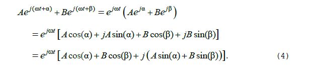
Then we convert the sum back to polar form as:

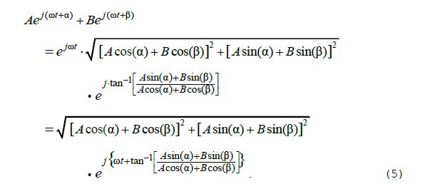
(The "•" symbol in Eq. (5), needed for text wraparound reasons, simply means multiply.) So, Eq. (5) tells us: the sum of two equal-frequency complex exponentials is merely a scalar magnitude factor multiplied by a unity-magnitude complex exponential term. Next we use Eq. (5) to obtain the expressions for the sum of two real-valued sinusoids.

The Sum of Two Cosine Functions
The following shows the derivation of the cosine expressions in Table 1. Equating the real parts of both sides of Eq. (5) yields the desired (but messy) equation for the sum of two arbitrary equal-frequency cosine functions as:

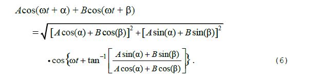
Eq. (6) is the general equation listed in the second row of Table 1. Substituting the different values for α, β, and B from the left column of Table 1 into Eq. (6), plus recalling just about every trigonometric identity known to the human race, allow us to obtain the expressions in the right column of the remaining rows in Table 1.

The Sum of Two Sine Functions
Equating the imaginary parts of both sides of Eq. (5) leads us to the desired equations for the sum of two general equal-frequency sine functions given in  Table 2.

The Sum of a Cosine Function and a Sine Function
We find the equation for the sum of a general cosine function and a general sine function, having the same frequencies, by recalling that sin(θ) = cos(θ – π/2) and using Eq. (6) as:

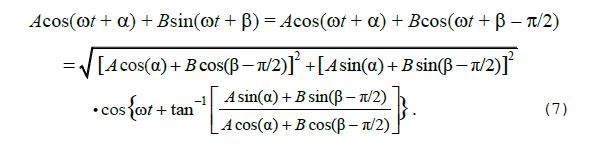
Knowing that cos(θ – π/2) = sin(θ) and sin(θ – π/2) = –cos(θ), we modify Eq. (7) as:

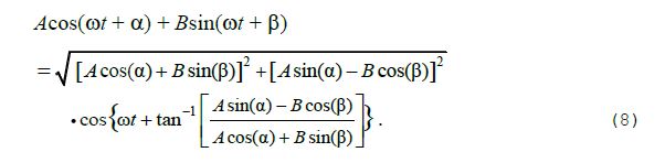
Eq. (8) is the general equation listed in the second row of Table 3. Substituting the different values for α, β, and B from the left column of Table 3 into Eq. (8), plus recalling the lots of trig identities, allow us to obtain the expressions in the right column of the remaining rows in Table 3.

Epilogue
As it turns out, the summation of two different-frequency sinusoids is also an interesting subject--more interesting than you might expect. If you have nothing better to do, have a look at my www.dsprelated.com blog titled: " Beat Notes: An Interesting Observation."

References
[1] McClellan, J., Schafer, R., Yoder, M., DSP First: A Multimedia Approach, Prentice Hall; Upper Saddle River, New Jersey, 1998, pp. 48-50.

[2] Smith, J., "A Sum of Sinusoids at the Same Frequency is Another Sinusoid at that Frequency", http://ccrma.stanford.edu/~jos/filters/Sum_Sinusoids_Same_Frequency.html.

[3] Smith, J., "Why Sinusoids are Important", http://www-ccrma.stanford.edu/~jos/mdft/Why_Sinusoids_Important.html.

[4] Anderson, J., Digital Transmission Engineering, 2/E, IEEE Press; Piscataway, New Jersey, 2005, pp. 288-289.

Sign in