On Nov 13, 11:45=A0am, pnachtwey <pnacht...@gmail.com> wrote:> On Nov 13, 6:44=A0am, RRogers <rerog...@plaidheron.com> wrote: > > > On Nov 12, 8:43=A0pm, pnachtwey <pnacht...@gmail.com> wrote: > > > > On Nov 11, 10:18=A0am, RRogers <rerog...@plaidheron.com> wrote: > > > > > On Nov 10, 11:54=A0am, Tim Wescott <t...@seemywebsite.com> wrote: > > > > > > On Tue, 10 Nov 2009 11:54:36 -0500, Datesfat Chicks wrote: > > > > > > "Frank W." <frankw_use...@mailinator.com> wrote in message > > > > > >news:7lggquF3dt584U1@mid.dfncis.de... > > > > > > >> Since all PID temperature controllers have Autotune, there mus=t be a> > > > > >> solution for this problem. Any ideas? > > > > > > > As you probably know from control theory, the basic theory of a=PID> > > > > > controller is that you have a system described by a set of line=ar> > > > > > differential equations that is inherently unstable or has some > > > > > > performance problems. =A0As a result you strap a PID controller=onto it> > > > > > (with said controller also described by its own linear differen=tial> > > > > > equations), and the resulting system (now described by linear > > > > > > differential equations which are a mathematical mix of the unde=rlying> > > > > > system and the PID controller) has better characteristics. > > > > > > > Did you notice that there is a word that appears many times in =my> > > > > > description above? > > > > > > > Want to guess what the word is? > > > > > > > That word is "linear". > > > > > > > A system with a time delay is not described by linear different=ial> > > > > > equations. =A0Strapping a PID controller onto it is bad math. > > > > > > > One of the more classic examples is a shower or an industrial p=rocess> > > > > > that mixes fluids of varying temperature and the sensor is loca=ted> > > > > > substantially downstream from the mixing value. =A0This is a pu=re time> > > > > > delay. =A0My shower at home is like that. =A0I turn the water a=little> > > > > > hotter. =A0Nothing happens. =A0I turn it a little more hotter. ==A0Nothing> > > > > > happens. =A0Then I turn it a little more hotter. =A0Then the wa=ve of hot> > > > > > liquid hits me and I scream in agony. > > > > > > > Over time, I've adapted to my shower. =A0I don't burn myself an=ymore.> > > > > > > I think the control algorithms you want to use for a system lik=e yours> > > > > > fall outside the range of PID. =A0I'm sure there is a body of t=heory that> > > > > > covers it, but I don't know what that is. > > > > > > > I would heat the system full bore for a fixed period of time, t=hen stop> > > > > > and wait to see how the temperature catches up. =A0And work fro=m there.> > > > > > > The best control strategy for that system isn't going to be PID=. =A0That> > > > > > is a non-linear system. > > > > > > I've been resisting forking this over into the control newsgroup:=now> > > > > it's compelling. > > > > > > Systems with delay can be perfectly linear, as well as time invar=iant --> > > > > they just can't be described by ordinary differential equations w=ith a> > > > > finite number of states. > > > > > > To be linear, a system only needs to satisfy the superposition pr=operty. =A0> > > > > A delay element satisfies superposition just fine. > > > > > > And while a PID controller may not be the theoretically best cont=roller> > > > > for a system with delay, in many cases it's not a bad choice at a=ll. =A0PID> > > > > controllers can and will give perfectly satisfactory service with=plants> > > > > that have significant delay. =A0The thousands, if not millions, o=f PID> > > > > controllers in mills and factories around the world that are cont=rolling> > > > > plants whose responses are dominated by delay certainly belie any > > > > > declaration that the PID controller isn't a good choice to contro=l a> > > > > plant with delay. > > > > > > None of the above is intended to minimize the difficulty in analy=zing and> > > > > designing a truly optimal controller for a plant with pure delay =--> > > > > that's an exercise that can make your brain hurt, and fast. =A0An=d nothing> > > > > of the above is intended to chase you away from taking plant dela=ys more> > > > > directly into account if a discrete-state controller such as a PI=D won't> > > > > let you eke the performance that you need out of your plant. =A0 > > > > > > But in the absence of significant nonlinearities or time varying =behavior> > > > > you can use all the analysis tools that are suitable for linear t=ime> > > > > invariant systems on a system with delays just fine. =A0You can d=o good> > > > > design work, without ever having to explicitly write out the diff=erential> > > > > equations, much less solving them. > > > > > > So if you don't want to get lost in Mathemagic Land searching for > > > > > performance that isn't necessary for your product's success, a go=od ol'> > > > > PID controller may be exactly the optimal controller -- in terms =of> > > > > adequate performance and reasonable engineering time -- even if i=t> > > > > doesn't satisfy any egghead academic measure of "optimal" for the > > > > > particular plant you're trying to control. > > > > > > --www.wescottdesign.com > > > > > I have recently done a thermal MIMO =A0PID controller that ended up > > > > preforming adequately despite using very simple controls. > > > > Some comments: > > > > Even the simplest differential description ends up with an infinite > > > > number of state/poles. > > > > Most real thermal systems have little tabs and things that foul up > > > > theoretical analysis. > > > > Therefore: you can start with simple mathematical models to estimat=e> > > > requirements but you always end up with approximations. > > > > Pole zero analysis in this case is almost worthless except to rough=ly> > > > get started. > > > > Bode and/or Nichol's chart analysis (I used both) works very well; > > > > but .. > > > > You have to get and use the experimental data. =A0You can use that > > > > directly or find a sufficiently good model for the system. > > > > You should establish a "process" for the tuning and experiments; th=e> > > > system you take the data on will undoubtedly not be the one that en=ds> > > > up being manufactured. > > > > Gotcha's: =A0Scilab's system identification processes are unstable > > > > dealing with this type of system. =A0They can be used to attempt > > > > modelling but tread carefully and double check. > > > > When taking the data, the room/environmental temperature will do > > > > everything it can to confound the experiment. > > > > Don't worry about the lower frequencies, go to where the phase star=ts> > > > to shift significantly. > > > > For the Bode/Nichols derived compensation just redo the experiment > > > > (which you probably will) to clarify the standard compensation regi=on> > > > round the Bode criterion; 180 degrees +- one or two decades. > > > > Try to give at least hints to how the tuning was done for the > > > > "outsourced" maintenance people who have to maintain the tuning aft=er> > > > the mechanical assembly is altered; unless you want to come back an=d> > > > start over yourself in a year. > > > > > Really, really examine the code to make sure you don't "windup". ==A0 I> > > > was forced to rely on programmers in another group and I had study =the> > > > experimental results for a while to realize that the anti-windup co=de> > > > just clipped the output not the integrator. > > > > > Ray > > > > I agree with the last paragraph. > > > However, I have had a lot of success with identifying systems poles > > > and zero. =A0 I can then place both where I want with the controller > > > gains. > > > > I didn't know Scilab has a system identification function, but I have > > > used the lsqrsolve and optim successfully. > > > > Peter Nachtwey > > > Interesting, I have thought about going that route but opted for a > > more conventional process; =A0System Identification routines. =A0But th=at> > wasn't very satisfactory. =A0I have a problem in that I like to continu=e> > along routes until I really understand why they don't work. =A0Sometime=s> > I think that half my brain is autistic. > > Once I get my system identification code reorganized (with or without > > a gui) I plan to test it against my data and some available test cases > > from NICONET. =A0 Although they don't seem to be MIMO. =A0In biological > > testing equipment you are forced into MIMO situations in order get the > > required temperature accuracy over large testing areas and > > environmental conditions. =A0In addition mammalian reactions are tuned > > to constant temperature within a narrow band; 37degC in our case > > (presuming no aliens in the group). =A0 I was actually looking forward > > to doing that; I had never had use MIMO before. =A0Wasn't so enthused > > after a while; the design process is a lot more complicated and the > > tools were not robust. > > Once I resolve (or at least identify) the problems perhaps I will > > compare the results with lsqrsolve. =A0If your interested I will post a > > link here; but don't expect anything soon. =A0I am just settling into > > Mexico, and am not as fast as I used to be. > > > Ray > > When you have MIMO test data why don't you share it with us. =A0I would > like to have a crack at too. > It would be helpful to know what I am fitting data too though so I can > get the general form the equations right. =A0I don't know anything about > your field of study. > > The trick is how you use optim() and lsqrsolve(). The best system > identification uses Runge-Kutta to integrate the model's system of > differential equations. > > For MIMO systems you will need to use optim(). =A0optim() can optimize a > cost function. =A0lsqrsolve() requires two arrays of data, the actual > data and the estimated data. =A0I don't know how you would do this if > you have two sets of actual data and two sets of estimated data. > > Peter NachtweyI don't quite understand your approach; it seems different from what I had in mind. I have multiple sets of experimental data consisting of three stimulus/drive columns and three columns of resulting temerature data; together with a multitude of other columns of other temperature readings for thermal design of the overall assembly. My hypothetical approach to raw curve fitting type of modeling: Write out the ABCD equations with unknown coefficients and try to find the coefficients; which are linear (superficially) coefficients applied to the data. Having an adequate model in hand, then I thought I would use optim() to find the control gains in the closed loop. This is not what you are describing. My formulation was just a passing thought and certainly has a lot of problems I haven't resolved. Your comments don't fall in line with this, so why not tell me yours. Brief technical details follow (of interest only to those who enjoy these things): The system consists of three heaters and three sensors; actually far more sensors for the data, but the others were temporary and informational for the rest of the machine and not used in control. The system consists of a disk holding something like 20 test strips and rotating the strips under a dispenser and then under an optical head; so each of the test strips rotated to have a drop of sample deposited and then put under the optical head to monitor the reaction development. One of the heating systems was a buffer to isolate the test disk from the room. The other two are more precise and localized controls that control the sample tray fairly precisely to 37 degC. The reason for two heaters: one controls most of the circular sample disk consisting of 20 or so test strips that have been entered; the other heater brings the incoming test strips up to temperature from the room temperature when they are inserted. The original specs were that the samples had to be at 37degC +- .1degC when the reaction was occuring, warmup in 5 minutes, ambient/room temperature 18degC to 30degC. I designed the control system to be .02 degC accurate at the tray thermistor, control loop closure at power up inside of two minutes, PID controls around the principal MIMO directions (the thermistors were placed reasonably close to the individual heaters). The last part was to make the programming (done by another group) and maintenance easier; requiring less skilled people and the end performance was adequate. The problems involved were: 1) I couldn't put the thermistors where I actually wanted them, 2) I couldn't be hyper conservative and truly insulate the assembly ( the mechanical people had more than enough problems) so I had to rely on chunks of metal smoothing out the spatial frequencies. Of course the assembly had variations across it anyway. 3) I never had the final machine available during testing because the mechanical people needed to know about thermal problems before the design was finished, and I didn't want to be the person holding up release after the machine was finished. The was only a problem during testing since one set of readings would be different from a set taken later. 4) The sys-id routines were not robust and had to be watched very carefully. In fact I ended up using the DC gains of the models as the first quality determiner. Then I would look at various residuals to determine the real quality. Usually the test data was split in half (or so) so the model wouldn't be just regurgitating data back to me. The first half was used to determine a model and then the model was used to predict the second half; the resulting residual time series were then examined. I wanted the residuals to be below .1 degC (1 part out of 370) or so but never got there due to inadequacies in the model, and I had to settle for 2 degC; the slack/error was taken up when the loops were closed. Apparently the sys-id routines want random inputs; whereas people are more comfortable with large step inputs. I have both types of data. 5) All of the heater systems talk to each other and the environment thermally; the reason for MIMO approach. 6) Severe organizational problems with people who had never done instrument design before (: That's a different story. What is driven home is the fact that you are just looking for an adequate model of reality in thermal situations; not looking for "truth". The mechanical assembly can not reduced to anything less than a FEA analysis; which I couldn't get the department to institute. It's not a trivial thing to incorporate in a design process. Having done a partial survey I think COMSOL is a pretty good multiphysics tool and does have the ability to incorporate spice models between objects like a thermistor (actually a point) and a heater. And so on, I have more information. None of this relates to any proprietary information; except if I come up with a better process I can answer questions from the engineer who has to redo the system after they make changes to the mechanical design. The design changes are inevitable and occasionally people get back to me with questions. If you really want some data I can post it on an FTP sight. The project is done and I am retired so there is no hurry. The data is not clean and has a lot of confounding disturbances; OTOH there is a lot of it :) I am still interested in determining a better process for establishing good models; although I am inclined to fix up the sys- id functions so that higher order approximations don't lead to (wildly) worse and worse predictions. That is just nonsense. Be aware that my criteria are DC gain and residuals; and any comment on the modelling will probably be oriented around that. If your interested in my code; my SCILAB program does produce a lot of outputs, BODE and Nichols charts; but is not finished code in the sense that some parameters are done with I/O, and some parameters are entries in the code. There are shortcomings, I never did a good Bode plot of the raw data, just of the models. I kept meaning to but that requires a lot of filtering to be meaningful. Hope I haven't bored you to much Peter. Ray
PID autotuning - not working for heating application
Started by ●November 5, 2009
Reply by ●November 14, 20092009-11-14
Reply by ●November 14, 20092009-11-14
"RRogers" <rerogers@plaidheron.com> schrieb im Newsbeitrag news:d45695c8-7d48-4841-934f-6cf13d8dd4f2@f20g2000prn.googlegroups.com...> On Nov 13, 11:45 am, pnachtwey <pnacht...@gmail.com> wrote: >> On Nov 13, 6:44 am, RRogers <rerog...@plaidheron.com> wrote: >> >> > On Nov 12, 8:43 pm, pnachtwey <pnacht...@gmail.com> wrote: >> >> > > On Nov 11, 10:18 am, RRogers <rerog...@plaidheron.com> wrote: >> >> > > > On Nov 10, 11:54 am, Tim Wescott <t...@seemywebsite.com> wrote: >> >> > > > > On Tue, 10 Nov 2009 11:54:36 -0500, Datesfat Chicks wrote: >> > > > > > "Frank W." <frankw_use...@mailinator.com> wrote in message >> > > > > >news:7lggquF3dt584U1@mid.dfncis.de... >> >> > > > > >> Since all PID temperature controllers have Autotune, there >> > > > > >> must be a >> > > > > >> solution for this problem. Any ideas? >> >> > > > > > As you probably know from control theory, the basic theory of a >> > > > > > PID >> > > > > > controller is that you have a system described by a set of >> > > > > > linear >> > > > > > differential equations that is inherently unstable or has some >> > > > > > performance problems. As a result you strap a PID controller >> > > > > > onto it >> > > > > > (with said controller also described by its own linear >> > > > > > differential >> > > > > > equations), and the resulting system (now described by linear >> > > > > > differential equations which are a mathematical mix of the >> > > > > > underlying >> > > > > > system and the PID controller) has better characteristics. >> >> > > > > > Did you notice that there is a word that appears many times in >> > > > > > my >> > > > > > description above? >> >> > > > > > Want to guess what the word is? >> >> > > > > > That word is "linear". >> >> > > > > > A system with a time delay is not described by linear >> > > > > > differential >> > > > > > equations. Strapping a PID controller onto it is bad math. >> >> > > > > > One of the more classic examples is a shower or an industrial >> > > > > > process >> > > > > > that mixes fluids of varying temperature and the sensor is >> > > > > > located >> > > > > > substantially downstream from the mixing value. This is a pure >> > > > > > time >> > > > > > delay. My shower at home is like that. I turn the water a >> > > > > > little >> > > > > > hotter. Nothing happens. I turn it a little more hotter. >> > > > > > Nothing >> > > > > > happens. Then I turn it a little more hotter. Then the wave >> > > > > > of hot >> > > > > > liquid hits me and I scream in agony. >> >> > > > > > Over time, I've adapted to my shower. I don't burn myself >> > > > > > anymore. >> >> > > > > > I think the control algorithms you want to use for a system >> > > > > > like yours >> > > > > > fall outside the range of PID. I'm sure there is a body of >> > > > > > theory that >> > > > > > covers it, but I don't know what that is. >> >> > > > > > I would heat the system full bore for a fixed period of time, >> > > > > > then stop >> > > > > > and wait to see how the temperature catches up. And work from >> > > > > > there. >> >> > > > > > The best control strategy for that system isn't going to be >> > > > > > PID. That >> > > > > > is a non-linear system. >> >> > > > > I've been resisting forking this over into the control newsgroup: >> > > > > now >> > > > > it's compelling. >> >> > > > > Systems with delay can be perfectly linear, as well as time >> > > > > invariant -- >> > > > > they just can't be described by ordinary differential equations >> > > > > with a >> > > > > finite number of states. >> >> > > > > To be linear, a system only needs to satisfy the superposition >> > > > > property. >> > > > > A delay element satisfies superposition just fine. >> >> > > > > And while a PID controller may not be the theoretically best >> > > > > controller >> > > > > for a system with delay, in many cases it's not a bad choice at >> > > > > all. PID >> > > > > controllers can and will give perfectly satisfactory service with >> > > > > plants >> > > > > that have significant delay. The thousands, if not millions, of >> > > > > PID >> > > > > controllers in mills and factories around the world that are >> > > > > controlling >> > > > > plants whose responses are dominated by delay certainly belie any >> > > > > declaration that the PID controller isn't a good choice to >> > > > > control a >> > > > > plant with delay. >> >> > > > > None of the above is intended to minimize the difficulty in >> > > > > analyzing and >> > > > > designing a truly optimal controller for a plant with pure >> > > > > delay -- >> > > > > that's an exercise that can make your brain hurt, and fast. And >> > > > > nothing >> > > > > of the above is intended to chase you away from taking plant >> > > > > delays more >> > > > > directly into account if a discrete-state controller such as a >> > > > > PID won't >> > > > > let you eke the performance that you need out of your plant. >> >> > > > > But in the absence of significant nonlinearities or time varying >> > > > > behavior >> > > > > you can use all the analysis tools that are suitable for linear >> > > > > time >> > > > > invariant systems on a system with delays just fine. You can do >> > > > > good >> > > > > design work, without ever having to explicitly write out the >> > > > > differential >> > > > > equations, much less solving them. >> >> > > > > So if you don't want to get lost in Mathemagic Land searching for >> > > > > performance that isn't necessary for your product's success, a >> > > > > good ol' >> > > > > PID controller may be exactly the optimal controller -- in terms >> > > > > of >> > > > > adequate performance and reasonable engineering time -- even if >> > > > > it >> > > > > doesn't satisfy any egghead academic measure of "optimal" for the >> > > > > particular plant you're trying to control. >> >> > > > > --www.wescottdesign.com >> >> > > > I have recently done a thermal MIMO PID controller that ended up >> > > > preforming adequately despite using very simple controls. >> > > > Some comments: >> > > > Even the simplest differential description ends up with an infinite >> > > > number of state/poles. >> > > > Most real thermal systems have little tabs and things that foul up >> > > > theoretical analysis. >> > > > Therefore: you can start with simple mathematical models to >> > > > estimate >> > > > requirements but you always end up with approximations. >> > > > Pole zero analysis in this case is almost worthless except to >> > > > roughly >> > > > get started. >> > > > Bode and/or Nichol's chart analysis (I used both) works very well; >> > > > but .. >> > > > You have to get and use the experimental data. You can use that >> > > > directly or find a sufficiently good model for the system. >> > > > You should establish a "process" for the tuning and experiments; >> > > > the >> > > > system you take the data on will undoubtedly not be the one that >> > > > ends >> > > > up being manufactured. >> > > > Gotcha's: Scilab's system identification processes are unstable >> > > > dealing with this type of system. They can be used to attempt >> > > > modelling but tread carefully and double check. >> > > > When taking the data, the room/environmental temperature will do >> > > > everything it can to confound the experiment. >> > > > Don't worry about the lower frequencies, go to where the phase >> > > > starts >> > > > to shift significantly. >> > > > For the Bode/Nichols derived compensation just redo the experiment >> > > > (which you probably will) to clarify the standard compensation >> > > > region >> > > > round the Bode criterion; 180 degrees +- one or two decades. >> > > > Try to give at least hints to how the tuning was done for the >> > > > "outsourced" maintenance people who have to maintain the tuning >> > > > after >> > > > the mechanical assembly is altered; unless you want to come back >> > > > and >> > > > start over yourself in a year. >> >> > > > Really, really examine the code to make sure you don't "windup". >> > > > I >> > > > was forced to rely on programmers in another group and I had study >> > > > the >> > > > experimental results for a while to realize that the anti-windup >> > > > code >> > > > just clipped the output not the integrator. >> >> > > > Ray >> >> > > I agree with the last paragraph. >> > > However, I have had a lot of success with identifying systems poles >> > > and zero. I can then place both where I want with the controller >> > > gains. >> >> > > I didn't know Scilab has a system identification function, but I have >> > > used the lsqrsolve and optim successfully. >> >> > > Peter Nachtwey >> >> > Interesting, I have thought about going that route but opted for a >> > more conventional process; System Identification routines. But that >> > wasn't very satisfactory. I have a problem in that I like to continue >> > along routes until I really understand why they don't work. Sometimes >> > I think that half my brain is autistic. >> > Once I get my system identification code reorganized (with or without >> > a gui) I plan to test it against my data and some available test cases >> > from NICONET. Although they don't seem to be MIMO. In biological >> > testing equipment you are forced into MIMO situations in order get the >> > required temperature accuracy over large testing areas and >> > environmental conditions. In addition mammalian reactions are tuned >> > to constant temperature within a narrow band; 37degC in our case >> > (presuming no aliens in the group). I was actually looking forward >> > to doing that; I had never had use MIMO before. Wasn't so enthused >> > after a while; the design process is a lot more complicated and the >> > tools were not robust. >> > Once I resolve (or at least identify) the problems perhaps I will >> > compare the results with lsqrsolve. If your interested I will post a >> > link here; but don't expect anything soon. I am just settling into >> > Mexico, and am not as fast as I used to be. >> >> > Ray >> >> When you have MIMO test data why don't you share it with us. I would >> like to have a crack at too. >> It would be helpful to know what I am fitting data too though so I can >> get the general form the equations right. I don't know anything about >> your field of study. >> >> The trick is how you use optim() and lsqrsolve(). The best system >> identification uses Runge-Kutta to integrate the model's system of >> differential equations. >> >> For MIMO systems you will need to use optim(). optim() can optimize a >> cost function. lsqrsolve() requires two arrays of data, the actual >> data and the estimated data. I don't know how you would do this if >> you have two sets of actual data and two sets of estimated data. >> >> Peter Nachtwey > > I don't quite understand your approach; it seems different from what I > had in mind. I have multiple sets of experimental data consisting of > three stimulus/drive columns and three columns of resulting temerature > data; together with a multitude of other columns of other temperature > readings for thermal design of the overall assembly. > My hypothetical approach to raw curve fitting type of modeling: > Write out the ABCD equations with unknown coefficients and try to find > the coefficients; which are linear (superficially) coefficients > applied to the data. Having an adequate model in hand, then I thought > I would use optim() to find the control gains in the closed loop. > This is not what you are describing. My formulation was just a > passing thought and certainly has a lot of problems I haven't > resolved. > Your comments don't fall in line with this, so why not tell me yours. > > Brief technical details follow (of interest only to those who enjoy > these things): > The system consists of three heaters and three sensors; actually > far more sensors for the data, but the others were temporary and > informational for the rest of the machine and not used in control. > The system consists of a disk holding something like 20 test strips > and rotating the strips under a dispenser and then under an optical > head; so each of the test strips rotated to have a drop of sample > deposited and then put under the optical head to monitor the reaction > development. One of the heating systems was a buffer to isolate the > test disk from the room. The other two are more precise and localized > controls that control the sample tray fairly precisely to 37 degC. > The reason for two heaters: one controls most of the circular sample > disk consisting of 20 or so test strips that have been entered; the > other heater brings the incoming test strips up to temperature from > the room temperature when they are inserted. The original specs were > that the samples had to be at 37degC +- .1degC when the reaction was > occuring, warmup in 5 minutes, ambient/room temperature 18degC to > 30degC. I designed the control system to be .02 degC accurate at the > tray thermistor, control loop closure at power up inside of two > minutes, PID controls around the principal MIMO directions (the > thermistors were placed reasonably close to the individual heaters). > The last part was to make the programming (done by another group) and > maintenance easier; requiring less skilled people and the end > performance was adequate. The problems involved were: > 1) I couldn't put the thermistors where I actually wanted them, > 2) I couldn't be hyper conservative and truly insulate the assembly > ( the mechanical people had more than enough problems) so I had to > rely on chunks of metal smoothing out the spatial frequencies. Of > course the assembly had variations across it anyway. > 3) I never had the final machine available during testing because the > mechanical people needed to know about thermal problems before the > design was finished, and I didn't want to be the person holding up > release after the machine was finished. The was only a problem during > testing since one set of readings would be different from a set taken > later. > 4) The sys-id routines were not robust and had to be watched very > carefully. In fact I ended up using the DC gains of the models as the > first quality determiner. Then I would look at various residuals to > determine the real quality. Usually the test data was split in half > (or so) so the model wouldn't be just regurgitating data back to me. > The first half was used to determine a model and then the model was > used to predict the second half; the resulting residual time series > were then examined. I wanted the residuals to be below .1 degC (1 > part out of 370) or so but never got there due to inadequacies in the > model, and I had to settle for 2 degC; the slack/error was taken up > when the loops were closed. Apparently the sys-id routines want > random inputs; whereas people are more comfortable with large step > inputs. I have both types of data. > 5) All of the heater systems talk to each other and the environment > thermally; the reason for MIMO approach. > 6) Severe organizational problems with people who had never done > instrument design before (: That's a different story. > > What is driven home is the fact that you are just looking for an > adequate model of reality in thermal situations; not looking for > "truth". The mechanical assembly can not reduced to anything less > than a FEA analysis; which I couldn't get the department to > institute. It's not a trivial thing to incorporate in a design > process. Having done a partial survey I think COMSOL is a pretty good > multiphysics tool and does have the ability to incorporate spice > models between objects like a thermistor (actually a point) and a > heater. > > And so on, I have more information. None of this relates to any > proprietary information; except if I come up with a better process I > can answer questions from the engineer who has to redo the system > after they make changes to the mechanical design. The design changes > are inevitable and occasionally people get back to me with questions. > > If you really want some data I can post it on an FTP sight. The > project is done and I am retired so there is no hurry. The data is > not clean and has a lot of confounding disturbances; OTOH there is a > lot of it :) I am still interested in determining a better process > for establishing good models; although I am inclined to fix up the sys- > id functions so that higher order approximations don't lead to > (wildly) worse and worse predictions. That is just nonsense. > Be aware that my criteria are DC gain and residuals; and any comment > on the modelling will probably be oriented around that. If your > interested in my code; my SCILAB program does produce a lot of > outputs, BODE and Nichols charts; but is not finished code in the > sense that some parameters are done with I/O, and some parameters are > entries in the code. There are shortcomings, I never did a good Bode > plot of the raw data, just of the models. I kept meaning to but that > requires a lot of filtering to be meaningful. >See simple example with differential equation of order 2: * http://home.arcor.de/janch/janch/_control/20081123-real-system-model/ I try to find the best possible process transfer function (page 1) by using approximation methods on the basis of some measured values (page 2). Thereafter I have a benchmark test scheme (page 3) with a program (page 4) that automatically finds the best PID parameters using the IAE criteria. This could be done for process identifications up to differential equations of degree 6. -- Regards JCH
Reply by ●November 14, 20092009-11-14
clip..........> ... > > read more =BBOkay I have uploaded the file that corresponds to step inputs. This one is fairly clean. http://www.plaidheron.com/ray/temp static-test.jpg static-test.xls Should get you there. If there is a permission problem let me know; I will resolve. The .jpg is a graph to get the idea. T-11 is included to verify the environment didn't change much. The .xls is: sheet 1 graphs, sheet static-test is the long experimental run covering about 4 hours Cols: T-1,2,3 are the three direct thermistors used later for control Cols: M,N,O are the PWM drives, 0-100%, to the corresponding heaters; the trailing columns can be ignored The intermediate columns are various sensors distributed away from the actively controled points. Let me know and I (or you ) can cross-verify your model against other experimental runs. I have other experimental data sets that are less clear; some are basically random inputs to try to satisfy the sys-id programs. Ray
Reply by ●November 15, 20092009-11-15
"RRogers" <rerogers@plaidheron.com> schrieb im Newsbeitrag news:3d4e61d7-69d7-4431-a12a-88e31d5868f7@x5g2000prf.googlegroups.com...> clip.......... >> ... >> >> read more � > > Okay I have uploaded the file that corresponds to step inputs. This > one is fairly clean. > http://www.plaidheron.com/ray/temp > static-test.jpg > static-test.xls > Should get you there. If there is a permission problem let me know; I > will resolve. > > The .jpg is a graph to get the idea. T-11 is included to verify the > environment didn't change much. > The .xls is: sheet 1 graphs, sheet static-test is the long > experimental run covering about 4 hours > Cols: T-1,2,3 are the three direct thermistors used later for control > Cols: M,N,O are the PWM drives, 0-100%, to the corresponding heaters; > the trailing columns can be ignored > The intermediate columns are various sensors distributed away from the > actively controled points. > > Let me know and I (or you ) can cross-verify your model against other > experimental runs. > > I have other experimental data sets that are less clear; some are > basically random inputs to try to satisfy the sys-id programs. >Basically refering to * http://home.arcor.de/janch/janch/_control/20081123-real-system-model/ Can you approach the best possible ODE (process transfer function) in a range of order <= 6? C6 y'''''' + C5 y''''' + C4 y'''' + C3 y''' + C2 y'' + C1 y' + y = K Decimal commas! Example data points: 30 0 0 0,062 0 0,124 0,002 0,187 0,012 0,249 0,04 0,311 0,093 0,373 0,17 0,435 0,266 0,498 0,373 0,56 0,48 0,622 0,581 0,684 0,671 0,746 0,748 0,809 0,811 0,871 0,861 0,933 0,899 0,995 0,929 1,057 0,95 1,12 0,966 1,182 0,977 1,244 0,984 1,306 0,99 1,368 0,993 1,431 0,996 1,493 0,998 1,555 0,999 1,617 1 1,679 1 1,741 1 1,804 1,001 -- Regards JCH My solution see down here: Decimal commas! 1,048734E-06 y'''''' + 6,2427E-05 y''''' + 0,001548347 y'''' + 0,02048154 y''' + 0,1523982 y'' + 0,6047773 y' + y = 1,000953
Reply by ●November 15, 20092009-11-15
On Nov 14, 7:44=A0am, RRogers <rerog...@plaidheron.com> wrote:> I don't quite understand your approach; it seems different from what I > had in mind. =A0I have multiple sets of experimental data consisting of > three stimulus/drive columns and three columns of resulting temerature > data; together with a multitude of other columns of other temperature > readings for thermal design of the overall assembly. > =A0 =A0 =A0My hypothetical approach =A0to raw curve fitting type of model=ing:> Write out the ABCD equations with unknown coefficients and try to find > the coefficients; which are linear (superficially) coefficients > applied to the data. =A0Having an adequate model in hand, then I thought > I =A0would use optim() to find the control gains in the closed loop. > This is not what you are describing. =A0My formulation was just a > passing thought and certainly has a lot of problems I haven't > resolved. > Your comments don't fall in line with this, so why not tell me yours.Why not use the principle of superimposition. Test each heater with respect to each sensor and then find the FOPDT or SOPDT coefficients that work For the first temperature sensor you have a FOPDT formula that looks like t1'=3DA1*t1+B11*u1(t-dt11)+B12*u2(t-dt12)+B13*u3(t-dt13)+C Where: t1 is the temperature a sensor 1 A1 is the system time constant at temperature sensor 1. This is basically exp(-t/tau1). B11 is the input coupling of heater 1 to sensor 1. B12 is the input coupling of heater 2 to sensor 1. B13 is the input coupling of heater 3 to sensor 1. u1(t-dt11) is the heater 1 signal for time t. dt11 is the dead time from heater 1 to sensor 1. C is the ambient temperature. It had better be the same for all test unless the ambient temperature is really changing. It is easy to ID B11 B12 and B13 if they are turned on 1 at a time but the starting point should be ambient temperature or some steady state. When done you would have this t1'=3DA1*t1+B11*u1(t-dt11)+B12*u2(t-dt12)+B13*u3(t-dt13)+C t2'=3DA2*t2+B21*u1(t-dt21)+B22*u2(t-dt22)+B23*u3(t-dt23)+C t3'=3DA3*t3+B31*u1(t-dt31)+B32*u2(t-dt32)+B33*u3(t-dt33)+C All the coefficient could probably be ID at once but then it would be much harder to get exact values. It is best to do small sections at a time and rely on superimposition. The way I ID a system is like this http://www.deltamotion.com/peter/PDF/Mathcad%20-%20Sysid%20SOPDT.pdf 1. On page 1/10 I define the ideal SOPDT system. I chose different value to to see how the well the system identification works under different conditions Notice that there is dead time and I don't assume all the poles are at the same location like others on this newsgroup. 2. At the bottom of page 2/10 I generate the test data that is later to be used for system identification. I add noise the to ideal data just to simulate reality a bit. The CO(t) function is a few steps. The function can be arbitrary but I have found that the excitation is critical to the identification. Dead times and time constants are determined more accurately if the are step or rapid changes. The gain and ambient coefficients are determined more accurate if the are steps at different levels. 3. One page 3/10 I plot and save the generated test data. I can post it on my FTP site for you to practice with. Notice that this data has dead time and two poles that aren't at the same location. I could have added more noise but the quasi-Newton method seems to filter it out well. 4. One page 4/10 the system identification is done. Mathcad's Minerr function can be like either Scilab's optim() function or lsqrsolve function depending on the option chosen. I chose the quasi-Newton optimization which is similar to the optim() function. Runge-Kutta is used to integrate the differential equation. The differential equation doesn't need to be linear. I could easily put a none linear term in there like one that changes the gain as a function of temperature. This happens with heat exchangers because of the LMTD. Fluid systems are often of the form v'=3Dg/m-K*v^2. It is easy to ID non linear system IF you know the general form of the equation and just need to ID the constants. Notice that the ID'd poles are closer together than the real poles. I have notice that system identification tends to ID the poles closer together than what they really are. Notice that I all ID a dead time and an ambient temperature. This is something that JCH does not do. At the bottom of the MSE(), mean squared error function, is where I calculate the mean squared error between the estimated temperature and the actual or test data temperature. The Minerr function adjusts Kp,t1,t2,thetap, and C till the MSE is minimized. You can see the results are not perfect but that is reality. 5. On page 5/10 the actual or perfect response is compare to the estimated response. The response looks close, almost identical, even though the system identification puts the estimated poles closer together. Also notice that a good system identification routine can ID systems that are excited by more than just a step change. In fact they must must be able to do system identification with arbitrary excitation. Above I said the excitation is the key to doing system identification. One key is the make multiple steps at different levels. This is very important in computing the gain and computing the gain when it isn't linear. Heat exchanger's gain changes because of LMTD. ( log mean temperature difference ). 6. On page 6/10 PID gains are calculated using the estimated plant parameters found by system identification. My formula is a little more complex that the IMC formulas but the response is faster/better for the same closed loop time constant. I doubt the extra complexity in the formula is worth the effort for most applications. 7 Page 7/10 simulates the PID control of the original system using the gains calculated from the system identification. Notice that feed back noise is simulated as well as the dead time. 8. Page 8/10. The simulation show the response. The response isn't perfect because there was noise in the original data used to do the system identification. The system identification is not perfect because the poles are closer together than they should be and I simulated noise on the feedback but this is closer to reality. 9 Page 9/10 uses the internal model gain formulas that I got from the www.controguru.com site. They work well too and are much simpler they don't work quite as mine. I should have provided a IAE value for my gains and the IMC gains for comparison. 10 page 10/10 shows the IMC response is a little slower but most would be please with it. I would use the above technique one at time with each heater and temperature sensor. Actually one can excite each of the heaters one at a time but the data for the 3 temperature sensors at the same time. I posted a link to a scilab program that does the same thing many years ago but no one seemed interested. JCH, you should copy this so your program can handle dead times, arbitrary inputs, and poles that are not all at the same place. What you appear to be missing the quasi-Newton code( BFGS) or Levenberg- Marquardt code that allows you to do proper optimization. I bet you use a grid search. Peter Nachtwey
Reply by ●November 15, 20092009-11-15
On Nov 14, 1:25=A0pm, RRogers <rerog...@plaidheron.com> wrote:> clip.......... > > > ... > > > read more =BB > > Okay =A0I have uploaded the file that corresponds to step inputs. =A0This > one is fairly clean.http://www.plaidheron.com/ray/temp > static-test.jpg > static-test.xls > Should get you there. =A0If there is a permission problem let me know; I > will resolve. > > The .jpg is a graph to get the idea. =A0T-11 is included to verify the > environment didn't change much. > The .xls is: sheet 1 graphs, sheet static-test is the long > experimental run covering about 4 hours > Cols: T-1,2,3 =A0are the three direct thermistors used later for control > Cols: M,N,O are the PWM drives, 0-100%, to the corresponding heaters; > the trailing columns can be ignored > The intermediate columns are various sensors distributed away from the > actively controled points. > > Let me know and I (or you ) can cross-verify your model against other > experimental runs. > > I have other experimental data sets that are less clear; some are > basically random inputs to try to satisfy the sys-id programs. > > RayWhen starting the identification process the system must be at steady state. The three temperature sensors are at different temperatures. That could be steady state for a combination of heater outputs but it is hard to know. If all the heaters started at the same ambient temperature then I know the system was at steady state. Peter Nachtwey
Reply by ●November 15, 20092009-11-15
On Nov 15, 6:14=A0am, "JCH" <ja...@nospam.arcornews.de> wrote:> "RRogers" <rerog...@plaidheron.com> schrieb im Newsbeitragnews:3d4e61d7-6=9d7-4431-a12a-88e31d5868f7@x5g2000prf.googlegroups.com...> > > > > clip.......... > >> ... > > >> read more =BB > > > Okay =A0I have uploaded the file that corresponds to step inputs. =A0Th=is> > one is fairly clean. > >http://www.plaidheron.com/ray/temp > > static-test.jpg > > static-test.xls > > Should get you there. =A0If there is a permission problem let me know; =I> > will resolve. > > > The .jpg is a graph to get the idea. =A0T-11 is included to verify the > > environment didn't change much. > > The .xls is: sheet 1 graphs, sheet static-test is the long > > experimental run covering about 4 hours > > Cols: T-1,2,3 =A0are the three direct thermistors used later for contro=l> > Cols: M,N,O are the PWM drives, 0-100%, to the corresponding heaters; > > the trailing columns can be ignored > > The intermediate columns are various sensors distributed away from the > > actively controled points. > > > Let me know and I (or you ) can cross-verify your model against other > > experimental runs. > > > I have other experimental data sets that are less clear; some are > > basically random inputs to try to satisfy the sys-id programs. > > Basically refering to > > *http://home.arcor.de/janch/janch/_control/20081123-real-system-model/ > > Can you approach the best possible ODE (process transfer function) in a > range of order <=3D 6? > > C6 y'''''' + C5 y''''' + C4 y'''' + C3 y''' + C2 y'' + C1 y' + y =3D K > > Decimal commas! > > Example data points: 30 > > 0 0 > 0,062 0 > 0,124 0,002 > 0,187 0,012 > 0,249 0,04 > 0,311 0,093 > 0,373 0,17 > 0,435 0,266 > 0,498 0,373 > 0,56 =A00,48 > 0,622 0,581 > 0,684 0,671 > 0,746 0,748 > 0,809 0,811 > 0,871 0,861 > 0,933 0,899 > 0,995 0,929 > 1,057 0,95 > 1,12 =A00,966 > 1,182 0,977 > 1,244 0,984 > 1,306 0,99 > 1,368 0,993 > 1,431 0,996 > 1,493 0,998 > 1,555 0,999 > 1,617 1 > 1,679 1 > 1,741 1 > 1,804 1,001 > > -- > Regards JCH > > My solution see down here: > > Decimal commas! > 1,048734E-06 y'''''' + 6,2427E-05 y''''' + 0,001548347 y'''' + 0,02048154 > y''' + 0,1523982 y'' + 0,6047773 y' + y =3D 1,000953We seem to have a disconnect here. The system is MIMO which means that a finite model would have a set of simultaneous differential equations. In my case three independent variables drives and three dependent variables; leading to three simultaneous differential equations whose order varies with the number of state variables needed for an adequate description. Including the room temperature we actually have four drives. Including the various components inside the instrument (motors, solenoids, and doors) we would have more; but for the sake of simplicity I took 3 drives and 3 sensors and treated the other drives as disturbances. A design assumption that could have been rendered wrong by results; but then I would have had to add more sensors and possibly more heaters. The reason for the 3 heaters and sensors is to establish control over extended mechanical assemblies having basically an infinite numbers of internal states. Although the higher order states are rapidly suppressed by the heat equation when the metal thermal time constant is short. As an illustration: The simple case of the sun warming a piece of ground through the seasons. The result is basically that a 20 degC surface variation causes .5 degC variation 2 meters down with a six month lag; with the transfer function having an infinite number of poles and a continuously rolling phase shift going through 180 deg over and over. This imposes constraints when you are trying to hurry it up via control systems. These numbers are "representative" since I am remembering; I do have the book Bell Labs book somewhere that solves the equation. Alternately: Writing the Green's function for the internal temperature of a bar heated at the surfaces requires an infinite degree polynomial resulting in an infinite number of poles in the Laplace xform. But the significance of higher poles drops down exponentially, so they don't matter unless you try to wrap a control loop and close the loop with time constants that are comprable. And so on Ray
Reply by ●November 15, 20092009-11-15
On Nov 15, 8:12=A0am, pnachtwey <pnacht...@gmail.com> wrote:> On Nov 14, 7:44=A0am, RRogers <rerog...@plaidheron.com> wrote:> I don't q=uite understand your approach; it seems different from what I> > had in mind. =A0I have multiple sets of experimental data consisting of > > three stimulus/drive columns and three columns of resulting temerature > > data; together with a multitude of other columns of other temperature > > readings for thermal design of the overall assembly. > > =A0 =A0 =A0My hypothetical approach =A0to raw curve fitting type of mod=eling:> > Write out the ABCD equations with unknown coefficients and try to find > > the coefficients; which are linear (superficially) coefficients > > applied to the data. =A0Having an adequate model in hand, then I though=t> > I =A0would use optim() to find the control gains in the closed loop. > > This is not what you are describing. =A0My formulation was just a > > passing thought and certainly has a lot of problems I haven't > > resolved. > > Your comments don't fall in line with this, so why not tell me yours. > > Why not use the principle of superimposition. =A0 Test each heater with > respect to each sensor > and then find the FOPDT or SOPDT coefficients that work > For the first temperature sensor you have a FOPDT formula that looks > like > t1'=3DA1*t1+B11*u1(t-dt11)+B12*u2(t-dt12)+B13*u3(t-dt13)+C > Where: > t1 is the temperature a sensor 1 > A1 =A0is the system time constant at temperature sensor 1. =A0This is > basically exp(-t/tau1). > B11 is the input coupling of heater 1 to sensor 1. > B12 is the input coupling of heater 2 to sensor 1. > B13 is the input coupling of heater 3 to sensor 1. > u1(t-dt11) is the heater 1 signal for time t. > dt11 is the dead time from heater 1 to sensor 1. > C is the ambient temperature. =A0It had better be the same for all > test unless the ambient temperature is really changing. > It is easy to ID B11 B12 and B13 if they are turned on 1 at > a time but the starting point should be ambient temperature or > some steady state. When done you would have this > t1'=3DA1*t1+B11*u1(t-dt11)+B12*u2(t-dt12)+B13*u3(t-dt13)+C > t2'=3DA2*t2+B21*u1(t-dt21)+B22*u2(t-dt22)+B23*u3(t-dt23)+C > t3'=3DA3*t3+B31*u1(t-dt31)+B32*u2(t-dt32)+B33*u3(t-dt33)+C > > All the coefficient could probably be ID at once but then it would > be much harder to get exact values. It is best to do small sections > at a time and rely on superimposition. > > The way I ID a system is like thishttp://www.deltamotion.com/peter/PDF/Ma=thcad%20-%20Sysid%20SOPDT.pdf> > 1. On page 1/10 I define the ideal SOPDT system. =A0I chose different > value to to see how the well the system identification works under > different conditions Notice that there is dead time and I don't assume > all the poles are at the same location like others on this newsgroup. > 2. At the bottom of page 2/10 I generate the test data that is later > to be used for system identification. =A0I add noise the to ideal data > just to simulate reality a bit. =A0The CO(t) function is a few steps. > The function can be arbitrary but I have found that the excitation is > critical to the identification. =A0 Dead times and time constants are > determined more accurately if the are step or rapid changes. =A0The gain > and ambient coefficients are determined more accurate if the are steps > at different levels. > 3. One page 3/10 I plot and save the generated test data. =A0I can post > it on my FTP site for you to practice with. =A0Notice that this data has > dead time and two poles that aren't at the same location. =A0I could > have added more noise but the quasi-Newton method seems to filter it > out well. > 4. One page 4/10 the system identification is done. =A0Mathcad's Minerr > function can be like either Scilab's optim() function or lsqrsolve > function depending on the option chosen. =A0I chose the quasi-Newton > optimization which is similar to the optim() function. =A0Runge-Kutta is > used to integrate the differential equation. The differential equation > doesn't need to be linear. =A0I could easily put a none linear term in > there like one that changes the gain as a function of temperature. > This happens with heat exchangers because of the LMTD. =A0Fluid systems > are often of the form > v'=3Dg/m-K*v^2. =A0It is easy to ID non linear system IF you know the > general form of the equation and just need to ID the constants. > Notice that the ID'd poles are closer together than the real poles. =A0I > have notice that system identification tends to ID the poles closer > together than what they really are. =A0Notice that I all ID a dead time > and an ambient temperature. =A0This is something that JCH does not do. > At the bottom of the MSE(), mean squared error function, is where I > calculate the mean squared error between the estimated temperature and > the actual or test data temperature. The Minerr function adjusts > Kp,t1,t2,thetap, and C till the MSE is minimized. =A0You can see the > results are not perfect but that is reality. > 5. On page 5/10 the actual or perfect response is compare to the > estimated response. =A0The response looks close, almost identical, even > though the system identification =A0puts the estimated poles closer > together. =A0Also notice that a good system identification routine can > ID systems that are excited by more than just a step change. =A0In fact > they must must be able to do system identification with arbitrary > excitation. =A0 Above I said the excitation is the key to doing system > identification. =A0 One key is the make multiple steps at different > levels. =A0This is very important in computing the gain and computing > the gain when it isn't linear. =A0 Heat exchanger's gain changes because > of LMTD. ( log mean temperature difference ). > 6. On page 6/10 PID gains are calculated using the estimated plant > parameters found by system identification. =A0My formula is a little > more complex that the IMC formulas but the response is faster/better > for the same closed loop time constant. =A0I doubt the extra complexity > in the formula is worth the effort for most applications. > 7 Page 7/10 simulates the PID control of the original system using the > gains calculated from the system identification. =A0 Notice that feed > back noise is simulated as well as the dead time. > 8. Page 8/10. =A0The simulation show the response. =A0The response isn't > perfect because there was noise in the original data used to do the > system identification. =A0The system identification is not perfect > because the poles are closer together than they should be and I > simulated noise on the feedback but this is closer to reality. > 9 Page 9/10 uses the internal model gain formulas that I got from thewww.=controguru.comsite. =A0They work well too and are much simpler they> don't work quite as mine. =A0 I should have provided a IAE value for my > gains and the IMC gains for comparison. > 10 page 10/10 shows the IMC response is a little slower but most would > be please with it. > > I would use the above technique one at time with each heater and > temperature sensor. =A0 Actually one can excite each of the heaters one > at a time but the data for the 3 temperature sensors at the same time. > > I posted a link to a scilab program that does the same thing many > years ago but no one seemed interested. > > JCH, you should copy this so your program can handle dead times, > arbitrary inputs, and poles that are not all at the same place. What > you appear to be missing the quasi-Newton code( BFGS) or Levenberg- > Marquardt code that allows you to do proper optimization. =A0I bet you > use a grid search. > > Peter NachtweyPeter, Sorry I didn't answer earlier; I was answering JCH and putting the data up. I considered the route you illustrated, and perhaps I should have tried harder. But in your example in the above text you implicitly assumed (by writing the equation that way) that a good description was accessible through a single state variable per heater/ sensor, and I ran into intellectual problems trying to have the flexibility for extension. I did read your earlier posting and will reread it. The problem I had was this: Suppose the correct set of terms for sensor one was: x'=3DAx+Bu y=3DCx+Du Where u is heater power, y is the sensor readings, and x is the internal state vector larger than u or y . Now a set of individual SISO readings and using supposition would result in individual state vectors xi and Ai,Bi,Ci,Di . Some the state vectors might be shared between the individual responses and some not. How do you determine which ones are shared or not? I am sure I can make up a circuit with discrete components that would illustrate this. This interpretation problem could be resolvable, but I didn't see how to do it. If I am missing your point please post an example with more state variables. It does seem as though some generalization of Thevin's equivalence circuit theorem might be possible and applicable. Maybe using Telegin's theorem? But these thoughts are just meanderings of my mind. Ray
Reply by ●November 15, 20092009-11-15
On Nov 15, 8:17=A0am, pnachtwey <pnacht...@gmail.com> wrote:> On Nov 14, 1:25=A0pm, RRogers <rerog...@plaidheron.com> wrote: > > > clip.......... > > > > ... > > > > read more =BB > > > Okay =A0I have uploaded the file that corresponds to step inputs. =A0Th=is> > one is fairly clean.http://www.plaidheron.com/ray/temp > > static-test.jpg > > static-test.xls > > Should get you there. =A0If there is a permission problem let me know; =I> > will resolve. > > > The .jpg is a graph to get the idea. =A0T-11 is included to verify the > > environment didn't change much. > > The .xls is: sheet 1 graphs, sheet static-test is the long > > experimental run covering about 4 hours > > Cols: T-1,2,3 =A0are the three direct thermistors used later for contro=l> > Cols: M,N,O are the PWM drives, 0-100%, to the corresponding heaters; > > the trailing columns can be ignored > > The intermediate columns are various sensors distributed away from the > > actively controled points. > > > Let me know and I (or you ) can cross-verify your model against other > > experimental runs. > > > I have other experimental data sets that are less clear; some are > > basically random inputs to try to satisfy the sys-id programs. > > > Ray > > When starting the identification process the system must be at steady > state. =A0The three temperature sensors are at different temperatures. > That could be steady state for a combination of heater outputs but it > is hard to know. =A0If all the heaters started at the same ambient > temperature then I know the system was at steady state. > > Peter NachtweyPeter, Okay, I will post that experiment but it's not as clean. Since I only had shared access to the prototype I couldn't let the machine cool down long enough for a real restart, and (of course) the room temperature changed. These thermal systems have really long "tails"; some sections (plastic) absorb heat and let it out very slowly. Ray