How to Estimate Encoder Velocity Without Making Stupid Mistakes: Part I

Here's a common problem: you have a quadrature encoder to measure the angular position of a motor, and you want to know both the position and the velocity. How do you do it? Some people do it poorly -- this article is how not to be one of them.

Well, first we need to get position. Quadrature encoders are incremental encoders, meaning they can only measure relative changes in position. They produce a pair of pulse trains, commonly called A and B, that look like this:

You need two of them in order to distinguish between forward and reverse motion. If you need to know absolute position, you can buy a 3-channel encoder, with A and B signals and an index channel that produces a pulse once per revolution in order to signal where a reference position is.

A state machine can be used to examine the A and B pulses and produce up/down counts to a counter of arbitrary width, and the index pulse can be used to initialize the counter to 0 at startup. There are some subtleties here involving noise and failure modes, but let's ignore them, for this article at least.

Most microcontrollers either have built-in encoder peripherals, or interrupt-on-input-change, or both. If you don't have an encoder peripheral, you have to examine the signals yourself and increment/decrement a counter. In any case, let's assume you can get a position count value which is correct based on the encoder signals. Our problem becomes one of taking samples of the position counter and estimating velocity.

Here's a concrete example. Let's consider an object that's rotating but slowing down exponentially due to viscous drag. Here's what the position might look like:

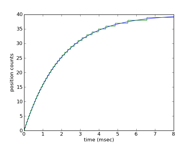
Here we show the actual continuous position of the object (converted to encoder counts), and the quantized position indicated by the encoder output. Quantized? Yes, both incremental and absolute encoders aredigital and have a quantizing effect. A quadrature encoder advertised as "256 lines" or "256 ppr" (pulses per revolution) measures 1024 counts per revolution: quadrature encoders yield 4 counts per cycle, and each cycle corresponds to a "line" (dark mark in an optical encoder) or a pulse measured on an oscilloscope.

In any case, we have lots of choices to obtain velocity from the position count.

The simplest approach is to estimate velocity = Δpos/Δt: measure the change in position and divide by the change in time. There are two classic options here:

• execute code at fixed time increments (constant Δt), measure position, and take Δpos = the difference between two successive position measurements
• execute code triggered by changes in encoder count (constant Δpos), measure elapsed time, and take Δt = the difference between two successive time measurements

The usual explanation is that the first approach (constant Δt) is better for moderate speeds and the second approach (constant Δpos) is better for low speeds. Texas Instruments has a user's guide (SPRUG05A) discussing this in detail:

It goes on to say:

At low speed, Equation 2 provides a more accurate approach. It requires a position sensor that outputs a fixed interval pulse train, such as the aforementioned quadrature encoder. The width of each pulse is defined by motor speed for a given sensor resolution.

[Cue buzzer sound] WRONG!!!!!!!

The rest of this article will be about understanding why that statement is wrong, why the constant Δpos approach is a poor choice, and (in part II) some more advanced algorithms for estimating position.

First we have to understand what would drive someone to choose the constant Δpos approach. The key to doing so lies in the second sentence I quoted above: "It requires a position sensor that outputs a fixed interval pulse train, such as the aforementioned quadrature encoder." If you have a pair of constant frequency square waves in quadrature, and you measure the encoder position in code executing at regular intervals, you might see something like this:

The bottom two waveforms are square waves with a frequency of 1618.03Hz = period of 0.61803 milliseconds (encoder count interval of 1/4 that = 0.154508 milliseconds = 6472.13Hz). The top two waveforms are those same waveforms but sampled at 0.1 millisecond intervals.

You'll note that the time between encoder state changes perceived by those sampled waveforms varies irregularly between 0.1 millisecond and 0.2 millisecond -- as it should be; we can't possibly measure 0.154508 millisecond intervals accurately, with code that executes at 0.1 millisecond granularity. Code that uses the constant Δt approach to measure velocity, with Δt = 0.1 milliseconds, would measure a velocity of either 0 or 10000Hz for this waveform at each sampling interval. The velocity resolution, for code that uses calculates Δpos/Δt using constant Δt, is 1/Δt.

This leads to three usual impulses:

1. Why don't I just use a larger Δt? Then my velocity resolution is smaller.
2. Why don't I just use a low-pass filter on the Δpos/Δt calculations?
3. Why don't I just use the constant Δpos approach?

We'll discuss the first two of these later. The constant Δpos approach (i.e. get interrupts at each encoder state change and measure the time), for fixed frequency waveforms, is actually the optimal approach. If I have a timer with 0.1 microsecond accuracy, and I get an interrupt on each encoder state change, then my resolution for velocity is not constant, like the constant Δt approach, but instead depends on the frequency. For this particular set of waveforms representing an encoder state frequency of 0.154508 milliseconds per state change, a 0.1 microsecond timer resolution would either measure 0.1545 or 0.1546 milliseconds between state changes = 6472.5Hz or 6468.3Hz -- for a velocity resolution of about 4.2Hz. The slower our waveforms, the more precise our velocity resolution can be using the constant Δpos approach.

What's wrong with that?

Well, for one thing, as the waveforms get faster, the precision gets worse, and the more interrupts we would get, leading to increased CPU usage. There's also the case of vibration around zero speed: you then have to distinguish between positive and negative position changes, and the velocity estimates in that case may be excessive. Those problems are pretty obvious.

The more subtle issue here is that the optimalness of the constant Δpos approach is true only for fixed frequency waveforms. If the frequency varies with time in an unknown manner, the constant Δpos approach only gives us the average frequency between instants at which the encoder state changes, which may not be what we want. I also said "the slower our waveforms, the more precise our velocity resolution can be" -- and precise is not the same as accurate.

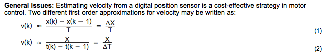
Let's go back do our earlier example of exponential decay. 

Here's what an estimated velocity waveform looks like when using the constant Δpos approach:

The blue is the actual velocity during this time, and the green is the estimated velocity. Notice how the green waveform is always above the blue waveform. In general this is always true, due to the backward-looking property of any real algorithm: when velocity is decreasing, any estimate of velocity will lag behind and be too high, and when velocity is increasing, any estimate of velocity will lag behind and be too low.

Now remember we only update the estimate when we get a change in encoder position. This is a problem with the constant Δpos approach. Suppose an object we're measuring is moving along at a certain slow but constant positive velocity: the encoder count updates periodically, and we'll calculate this velocity correctly. Now the object stops. No more encoder counts. But until we get another count, we won't update the velocity estimate! We never estimate a velocity of zero! We can "fix" this problem with a hack: set a timeout and when the timeout expires, estimate a velocity of zero. These sorts of fixes in signal processing are generally very bad: they're hard to analyze and you can't predict when the fix is going to backfire.

Aside from the zero velocity problem, the issue in general is due to the area between the two waveforms: actual and estimated velocity. In a good velocity estimator, this area will always be bounded by a number that's proportional to the acceleration rate. Here the area is larger the closer we get to zero velocity. Why do we care? Because the area is the integral of velocity, which is position: if you integrate the velocity estimate over time, you should get back the same value of position as you started with. The constant Δpos approach does not produce bounded position drift when you integrate the velocity estimate to obtain position. Does this matter in all systems? No, but it has consequences whenever you're using integrals of estimated velocity, for example in a PI controller.

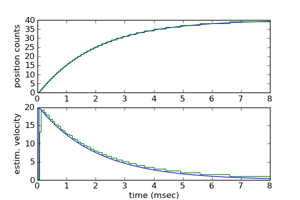
Another closely related issue is the time at which velocity estimates are obtained: they aren't at constant time intervals, but rather occur at each change in position count. Aside from the inconvenience of getting lots of interrupts at unpredictable times with high velocities, this means that they're not directly compatible with regularly-sampled control systems. There's a lot of valuable theory behind a control system that executes at regular intervals, and there are few reasons to deviate from this approach. If you have a PI controller that runs at regular intervals, and it gets velocity estimates from the constant Δpos approach, there will always be a time delay between the velocity estimate update, and the point in time at which it is used: the velocity estimate is effectively resampled at the rate at which it's used. This time delay is not constant and causes additional area between the real and estimated velocity waveforms:

It's not much but it causes additional error. (Look closely at this graph and the previous one.)

All of this discussion so far has assumed one thing about the encoder: that it's a perfect measuring device. We've quantized the real position into exactly equal intervals. A real position encoder has errors due to manufacturing tolerances.

The main mistake of using the constant Δpos approach is assuming an encoder is perfect. It's not. Let's look at an encoder I've used before, the Avago HEDS-55xx/56xx series. If you look at p. 4-6 of the datasheet, you'll see specifications, diagrams, and definitions for the errors in the encoder waveforms. Here are the position accuracy specifications:

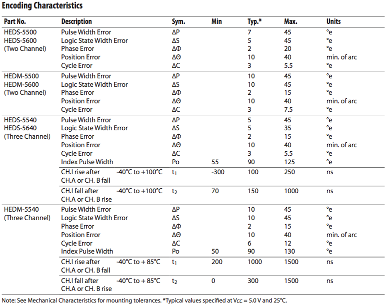
The encoder with the best specifications here is the HEDS-5540/5640 encoder, which specifies state width error ΔS = 35 degrees electrical maximum, 5 degrees typical. What does this mean for us if we're using the Δpos approach to estimate velocity?

Each encoder state is nominally 90deg electrical, so a ±35 degrees electrical error is a ±39% error; ±5 degrees electrical error is ±5.5% error. We calculate v = Δθ/Δt. The time measurement Δt is determined by the accuracy of the CPU clock, which for a crystal oscillator is typically 50ppm or less -- essentially negligible. So the error in velocity is directly proportional to the error in Δθ -- typically 5.5% and up to 39% error from one encoder state to the next!

We could use the time between each edge and the 4th-previous edge instead; this is the cycle time C specified in the datasheet. The error ΔC is 3 degrees typical, 5 degrees maximum -- with a 360 degree total cycle this works out to 0.8% typical, 1.4% maximum.

Note that these errors aren't DC errors, they appear as jitter from one state or one cycle to the next. So if we average these velocity estimates then the error is attenuated, which is fine for high speeds, but ruins the advantage of using the time between one encoder edge to the next -- but this is the whole point of using the constant Δpos approach!

So that's why I don't recommend using it. If you're using an encoder, and you can analyze the datasheet for it to determine the typical or worst-case errors, and you're fine with these numbers, then go ahead and use constant Δpos if you must.

Well, if constant Δpos is out, what's left?

Let's be fair and look at the constant Δt approach with the same kind of analysis. Here we must make an estimate. Let's assume the position count we measure represents the center of the encoder state. With a perfect encoder, sampling the position at any given instant can be off by up to 45 degrees electrical: the actual position could be at either edge of the pulse. This means that between two successive measurements we could be off by 90 degrees electrical.

Examples for which this is true: we make one measurement at the beginning of one encoder state, and the next measurement near the other end of that same encoder state, so the real change in position is 90 degrees electrical, and the estimated change in position is 0. Or we make one measurement just before the transition of an encoder state, and the other measurement just after the following transition, so the real change in position is 90 degrees and the estimated change in position is 2 counts = 180 degrees electrical. With an imperfect encoder that has a worst-case state width error of 35 degrees electrical, the worst-case value for real change in position in these two cases are 90+35 = 125 degrees electrical for an estimated change in position of 0, or 90-35 = 55 degrees electrical for an estimated change in position of 180 degrees; both cases add that worst-case error of the imperfect encoder, for a total worst-case error in Δpos of 125 degrees.

This error is a property of the encoder, not of the algorithm used.

The point I want to make here is that because encoders are imperfect, there will be a position error that we just have to expect and accept. With the constant Δt approach, this translates into a constant worst-case speed error, independent of speed. We have a choice of which Δt we want to use, which gets us back to two points I raised earlier:

1. Why don't I just use a larger Δt? Then my velocity resolution is smaller.
2. Why don't I just use a low-pass filter on the Δpos/Δt calculations?

The choice of Δt leads to a tradeoff. If we choose a large Δt, we get very low speed error, but we will also get a low bandwidth and large time lag. If we choose a small Δt, we get very high bandwidth and small time lag, but we will also have high speed estimation error.

If I were using the basic approach for estimating angular velocity, I would take the position estimates made at the primary control loop rate, take differences between successive samples, divide by Δt, and low-pass-filter the result with a time constant τ that reduces the bandwidth and error to the minimum acceptible possible. (A 1-pole or 2-pole IIR filter should suffice; if that kind of computation is expensive but memory is cheap, use a circular queue to store position of the last N samples and extend the effective Δt by a factor of N.)

If you're using the velocity estimate for measurement/display purposes, then you're all done. If you're using the velocity estimate for control purposes, be careful. It's better to keep filtering to a minimum and accept the velocity error as noise that will be rejected by the overall control loop performance.

Is the best we can do? Not quite. We'll discuss some more advanced techniques for velocity estimation in Part II of this article.