Signal Processing Contest in Python (PREVIEW): The Worst Encoder in the World
When I posted an article on estimating velocity from a position encoder, I got a number of responses. A few of them were of the form "Well, it's an interesting article, but at slow speeds why can't you just take the time between the encoder edges, and then...." My point was that there are lots of people out there which take this approach, and don't take into account that the time between encoder edges varies due to manufacturing errors in the encoder. For some reason this is a hard concept to accept. (Most of the other responses were "Where's Part II?" I apologize for the delay. More on this in a bit.)
And shortly after I wrote the article, I had an idea. I'm going to put my money where my mouth is, I thought, and have a contest. If someone thinks they can use the time between encoder instants, they'll just have to prove it! Ever since then, I've been trying to find the time to think up a tangible "bake-off" between encoder velocity estimation algorithms. I'm still working on it, but I've discussed my idea a little bit with Stephane Boucher, who runs this site, and I'm going to give you a preview of my contest proposal.
If you read this preview and are interested in participating, please send a quick comment to me so we can get a sense of how many people might participate.
The Contest, in brief:
You have the chance to come up with a good velocity estimation algorithm in Python, that processes information from a simulated quadrature encoder, and submit it to the contest. I'm going to evaluate your algorithm's accuracy, and the top entries will win some gift certificates to an electronics distributor like Digikey or Mouser. There will be at least 3 prizes, with values of at least $75 for the top prize. (That's if I'm sponsoring it on my own. If we can get enough interest, and Stephane can drum up some corporate sponsorship, we'd like to see it more in the $250 - $500 range.)
To make sure everything goes smoothly, it will still take a while to prepare. I'm aiming for final rules to be posted, and first entries accepted, on January 1, 2014, and last entries accepted 3 months later. (That gives you a 4-month head start if you read this preview!)
The Situation
You are an engineer at Shady Cybernetics, LLC, working on the motor controller for their next economy-model 5-axis robot arm. There's a lot of pressure to keep the price competitive. One of the other engineers, who's working on mechanical and manufacturing aspects of the arm, decided he was going to drop the Avago encoders you had during an early prototype. They're too expensive, he claims, and in their place, he's purchasing some knockoff encoders from a company in China you've never heard of, called Lucky Wheel Technology, Inc., which says they can meet the same specifications as the encoders from Avago, for half the price.
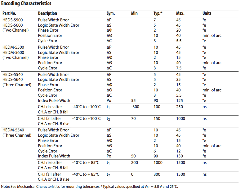
You are skeptical. Here are the accuracy specs from the HEDM-5540 encoders:

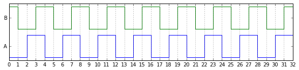
After taking a look at some samples from Lucky Wheel, you realize that they look pretty lousy. Here's what a perfect encoder's quadrature signals look like at constant speed:
Here's what some signals from one sample of the Lucky Wheel LW5540 look like:
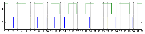
It's not just that the pulse widths are narrow or wide, or the quadrature angles are out of whack, it's that they're inconsistent. Look at the A signal around counts 2-5 and then around counts 26-28. The pulses are narrow at one point, and then a few counts later they're wide. But you make some careful measurements and crunch the numbers, and unfortunately they meet the specs, if just barely.
Before you spend a lot of time prototyping up some firmware on your embedded processor, you'd like to see how this affects your system design, so you digitize the encoder waveforms and then do some analysis with the Python scipy and numpy libraries.
The Rules
Contest submissions must meet the following rules (subject to change, since this is a preview**):
- Each submission must be a Python 2.7 file called
encoder_estimator.py - The file must be less than 65536 bytes in length.
- Your file may only contain imports of
scipyandnumpymodules; the imports must be in the first 20 lines of code before any other statements. (If you want to test your file, put your test harness in another script.) - Your file must include a Python class called
Estimatorwith theusesEdgeTimes(),onEdge(),estimatePosVel(), andgetPosVelScalingFactors()methods shown below. - Don't be evil: your file must not reference any double-underscore attributes, functions, or methods (except the
__init__()method in your user-defined classes), or reference or use any of Python's builtin functions except for those in an approved whitelist, which is TBD but will include at leastabs(),all(),any(),dict(),divmod(),enumerate(),float(),int(),iter(),len(),list(),long(),map(),max(),min(),object(),pow(),range(),round(),set(),slice(),sorted(),sum(),tuple(),xrange(), andzip(). - Any file that does not meet the above guidelines will be disqualified.
**Note: This can work in your favor — if you have a specific restriction you disagree with, and can convince me to relax the rules, I will do so. If there are Python modules not allowed by the above rules that you feel are necessary, let me know. I am looking at RestrictedPython as a sandboxing tool, but am still not sure that I want to permit the use of arbitrary Python code.
I will score your entry by running a test harness which instantiates your Estimator class and calls the following methods based on this interface, for a simulation time period of 5 seconds:
class Estimator(object):
    def usesEdgeTimes(self):
        '''Returns True or False:
        True if the estimator uses edge times, False if it does not.
        The caller may assume this function always returns the same answer.'''
        return True
    def onEdge(self, timeticks, count):
        '''Called at each edge, if usesEdgeTimes() returns True;
        timeticks is an integer in 10-nanosecond ticks
        count is an integer. No return value is necessary.'''
        pass
    def estimatePosVel(self, timetocks, count):
        '''Called at a 10kHz rate.
        timetocks is an integer in 100-microsecond tocks
        count is an integer.
        You should return a 2-element tuple containing a position and velocity
        estimate. Both position and velocity may be scaled to units of your choice.'''
        return (position, velocity)
    def getPosVelScalingFactors():
        '''You should return a 2-element tuple (posU, velU) containing
        position and velocity scaling factors. The results of estimatePosVel() are
        interpreted using these scaling factors: the product (position*posU)
        should be measured in mechanical revolutions, and the product (velocity*velU)
        should be measured in mechanical revolutions per second.'''
        return (posU, velU)
Your algorithm will be disqualified if it takes more time to run than a maximum time limit. The time limit will be a fixed multiple of the runtime of a reference algorithm (to be published). Please note that algorithms which use edge times are likely to run more slowly than algorithms that do not, since there are additional function calls. (If you return False from usesEdgeTimes(), the evaluation routine will not call onEdge().)
The system constraints
This system represents a 64-line encoder (256 counts per revolution) that meets the specifications for ΔP, ΔS, ΔPhi, and ΔC for the HEDM-5540.
Maximum velocity: ±6000RPM.
Maximum acceleration: ±15000RPM/sec. (Warning! This and the velocity limit may increase in the final rules.)
The starting velocity may be (and probably will be) nonzero.
Your algorithm will be evaluated for a simulated time of 5 seconds (50,000 calls to estimatePosVel()). You may assume that the encoder starts at position zero; don't worry about aligning to any position reference.
The velocity profile used for evaluation will be the same for all entries, but will not be revealed prior to posting the algorithm results.
Scoring
Points will be assigned to your algorithm based on the accuracy of position and velocity. [Method for evaluating TBD, but will probably be based on mean-squared error of velocity and position after filtering with a 1-pole 1msec time constant low-pass filter. See the section below.]
- You may submit multiple entries. (There may, however, be a limit applied if the total number of entries is large.)
- You may retain a copyright to your algorithm if you publish it under one of the following open-source licenses: Apache, BSD, MIT, ... [etc]. Submissions without a copyright notice are assumed to be submitted under the Apache license.
- You must submit your real name and your country and state/province of residence.
- The winning entries will be published on embeddedrelated.com
So that's the contest preview. Again, if you're interested in participating, send a quick comment to me.
How to test and evaluate an estimation algorithm
(or: How to Estimate Encoder Velocity Without Making Stupid Mistakes: Part 1.5)
The rest of this article will get into some technical information about position and velocity estimation. But first:
Mea Culpa: Why Jason Still Hasn't Published Part II
OK, so I set an expectation at the end of Part I of my article on encoder estimation that there would, in fact, be a Part II, and it would be on advanced estimation algorithms. I hinted on Reddit that it would cover some aspects of PLLs and observers.
Since then I've written eight other articles, so I can't exactly claim I haven't had time to write Part II. The toughest thing about writing a followup hasn't been the theory behind these advanced algorithms. What is tough to explain is what makes one algorithm better than another. And here I need to take a short diversion:
Over the years, I've read a lot of really good articles in IEEE Transactions. The journals I find most relevant are IEEE Transactions on Industrial Applications, IEEE Transactions on Industrial Electronics, and IEEE Transactions on Power Electronics. They have lots of papers on motor control, and a bunch of them are about current or flux or speed controllers. And I have some pet peeves. The first of which is that the editorial quality isn't very good. These are beautifully typeset professional journals which IEEE is investing a lot of money in. I am sure the editors are putting in the effort they can to make these journals better. But it appears like the only major criteria for getting an article published in these journals is that it first has to be presented in an IEEE conference, and beyond that, as long as the article meets certain minimum guidelines, the conference organizers nominate it for publication in the IEEE Transactions. This shuts out anyone who doesn't have the time or money to go to the conferences (and in industry, it's hard enough just getting the approval to publish something), and it lets through a lot of papers which, in my opinion, aren't very good. For me as a reader, it's not really that big of a deal, since I've read enough of them that I can quickly weed out the mediocre ones.
The second pet peeve is a more specific aspect of this, and it has to do with graphs. What I don't understand is why the editors don't have an acceptance threshold for graphs, involving some very simple criteria:
- All graphs should have their axes labeled, including engineering units. (you'd be surprised how many don't)
- Graphs showing more than one waveform should show clear distinguishing characteristics (e.g. line width, line style, and/or marker style), including a legend.
- Any graph meant to demonstrate small differences between waveforms must be accompanied by a graph showing that difference.
This last point may need some explanation. Here's an example of a bad graph.
import numpy as np
import matplotlib.pyplot as plt

x = np.arange(0.5,2,0.001)
f = lambda x: -0.09*x**2 + 0.68*x + 0.41
plt.plot(x,sqrt(x),x,f(x))
plt.title('Really cool approximation to $\sqrt{x}: f(x) = -0.09x^2 + 0.68x + 0.41$',
          fontsize=14)
plt.legend(('$\sqrt{x}$','$f(x)$'),'upper left')
plt.xlabel('x')
plt.ylabel('y')
plt.grid()
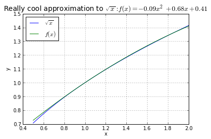
Why is it bad? Because you can't tell how close these two waveforms are! All I can tell is that, yeah, they're kind of close. Now watch what happens when you graph the error:
plt.plot(x,sqrt(x)-f(x))
plt.title('$\sqrt{x}-f(x)$')
plt.xlabel('x')
plt.ylabel('error')
plt.grid()
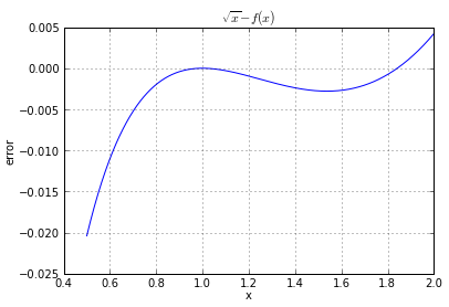
Bingo! I can immediately tell that the error is less than 0.005 between x = 0.7 and 2.0. And that's a lot more useful and a lot more specific than just knowing that \( f(x) \approx \sqrt{x} \).
The reason this is so crucial is that these are supposed to be rigorous papers explaining, and promoting, novel contributions to engineering. So many of them are saying, in effect, Here's Our Research And It Has The Potential To Improve The World! More specifically and more commonly, Our New (choose one or more of the following: Nonlinear, Adaptive, Robust, Lyapunov, \( H_\infty \), Recursive, Fuzzy Logic, Ant Colony, Neural Network) Control Algorithm Is An Improvement Over The Standard Proportional-Integral Controller! Which brings me to my third pet peeve:
The academic world needs to prevent the use of straw-man comparisons between new and standard techniques. Standard test cases should be developed for evaluating new methods. In the deceptive fields of politics and advertising, a straw man is a technique to portray an undesirable alternative inaccurately, thereby showing the contrast to a desirable alternative. In engineering papers, I don't think the authors are out to deceive people, but when they compare their new whiz-bang algorithm to a plain old PI controller, and you can see in the graph in their paper that their whiz-bang controller does a better job than the PI controller, the question you should be asking is, Hey, how do they really know they've done a good job tuning the PI controller? Just because one particular PI controller looks lousy in an application doesn't mean it's the best PI controller. And when I read about how Fuzzy Logic is supposed to be better, I have no way of knowing if that's really the case or whether the technique in question is just a thin improvement over a poorly-tuned PI controller for one particular test case. So I really, really, really wish that for these standard types of problems (field-oriented current control in PMSM motors, field-oriented current control in induction motors, direct torque control, etc., etc.) there were some standard test cases. And then the researchers could say "Our algorithm achieves a score of 145.3 on the Slawitsky Benchmark with test case E3, 182.3 with test case E4, and 167 with test case E5." And then you could get a better sense of why their research matters. I'm sorry if I'm devaluing the dissertations of Ph.D. students at the University of South Blahzistan here, but there's a difference between the value of someone's research to their university, and the value of their research to society as a whole. Go ahead and get your Ph.D. — you've earned it! — but I don't want to read about it unless it measures up to high standards.
Ride a Painted Pony, Let the Spinning Wheel Spin
OK, so let's do some measuring! We're going to choose one particular test case, with one particular UUT (unit under test, i.e. a consistent sample encoder behavior), and one particular algorithm, and see what happens.
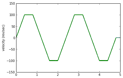
Let's create an acceleration/deceleration profile:
import scipy.integrate

t = np.arange(0,5,100e-6)
A0 = 15000.0/60
# max acceleration in rev/sec^2 = 15000RPM/sec
# acceleration waveform is zero except for a few intervals:
a = np.zeros_like(t)
a[t<0.4] = A0
a[(t>0.8) & (t<1.6)] = -A0
a[(t>2.0) & (t<2.8)] = A0
a[(t>3.2) & (t<4.0)] = -A0
a[(t>4.4) & (t<4.8)] = A0
omega_m = scipy.integrate.cumtrapz(a,t,initial=0)
theta_m = scipy.integrate.cumtrapz(omega_m,t,initial=0)

plt.figure(figsize=(8,6), dpi=80)
plt.subplot(3,1,1)
plt.plot(t,a)
plt.ylabel('accel (rev/sec^2)')

plt.subplot(3,1,2)
plt.plot(t,omega_m)
plt.ylabel('vel (rev/sec)')

plt.subplot(3,1,3)
plt.plot(t,theta_m % 1.0)
plt.ylabel('angle (rev)')
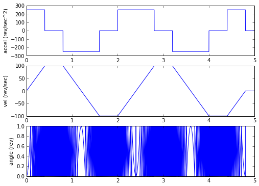
Yee hah! That was easy! Now we need our encoder.
So what exactly does an encoder look like in a signal processing chain? Well, if we lump it together with an encoder counter, we really just have a position quantizer.
class GenericEncoder(object):
    '''Subclasses must contain the field self.points
    which contains an array of the positions of all edge transitions.'''
    def getCountsPerRevolution(self):
        return len(self.points)
    def measureRaw(self, actualPos):
        '''here we want to support actualPos being an array'''
        positionInRevolution = np.array(actualPos) % 1.0
        numRevolutions = numpy.round(actualPos - positionInRevolution).astype(int)
        poscount = numpy.searchsorted(self.points, positionInRevolution)
        return (poscount, numRevolutions)
    def measure(self, actualPos):
        (poscount, numRevolutions) = self.measureRaw(actualPos)
        return poscount + numRevolutions * self.getCountsPerRevolution()

class PerfectEncoder(GenericEncoder):
    def __init__(self, N):
        self.points = np.arange(0,1,1.0/N)

class LuckyWheelEncoderUnit1(GenericEncoder):
    def __init__(self):
        self.points = np.array([
         1.78681261e-05,   4.34015460e-03,   8.07303047e-03,
         1.13466271e-02,   1.61623994e-02,   1.96503069e-02,
         2.31784992e-02,   2.64520959e-02,   3.17064152e-02,
         3.57948381e-02,   3.88021793e-02,   4.25872245e-02,
         4.76602727e-02,   5.13552252e-02,   5.46335835e-02,
         5.79334630e-02,   6.27657415e-02,   6.73314917e-02,
         7.07513269e-02,   7.40779942e-02,   7.78712102e-02,
         8.24369605e-02,   8.67480414e-02,   8.91834630e-02,
         9.33930296e-02,   9.79757390e-02,   1.02623678e-01,
         1.05065715e-01,   1.08709319e-01,   1.13081208e-01,
         1.18193111e-01,   1.21210246e-01,   1.24645388e-01,
         1.29050112e-01,   1.33366964e-01,   1.37354778e-01,
         1.40035335e-01,   1.44155580e-01,   1.48472433e-01,
         1.52460246e-01,   1.56179866e-01,   1.60160736e-01,
         1.64505892e-01,   1.68334854e-01,   1.71457270e-01,
         1.76305268e-01,   1.80495679e-01,   1.84137509e-01,
         1.87601801e-01,   1.92449799e-01,   1.95613191e-01,
         1.99748524e-01,   2.03746332e-01,   2.07555268e-01,
         2.11757722e-01,   2.15751676e-01,   2.18986641e-01,
         2.23067092e-01,   2.27068877e-01,   2.30992969e-01,
         2.34994386e-01,   2.38905898e-01,   2.42175623e-01,
         2.46098438e-01,   2.50440268e-01,   2.54696760e-01,
         2.58320154e-01,   2.61880090e-01,   2.66011140e-01,
         2.70211800e-01,   2.73425623e-01,   2.77786595e-01,
         2.81903811e-01,   2.85816794e-01,   2.88915751e-01,
         2.93357018e-01,   2.97671257e-01,   3.00922263e-01,
         3.05060282e-01,   3.09496091e-01,   3.12840812e-01,
         3.16027731e-01,   3.20358746e-01,   3.25116017e-01,
         3.28838087e-01,   3.32146173e-01,   3.36258477e-01,
         3.40221486e-01,   3.44538385e-01,   3.47806642e-01,
         3.51548143e-01,   3.55622481e-01,   3.59643853e-01,
         3.62912111e-01,   3.66904329e-01,   3.71767013e-01,
         3.75263736e-01,   3.79056642e-01,   3.82319633e-01,
         3.87423892e-01,   3.90882952e-01,   3.94162111e-01,
         3.97634225e-01,   4.03172934e-01,   4.07015722e-01,
         4.10025417e-01,   4.13672599e-01,   4.18413278e-01,
         4.22525788e-01,   4.25130886e-01,   4.28778068e-01,
         4.33518747e-01,   4.38513745e-01,   4.40961988e-01,
         4.44261170e-01,   4.49543367e-01,   4.53633247e-01,
         4.57106519e-01,   4.60405701e-01,   4.65019062e-01,
         4.68738715e-01,   4.72511159e-01,   4.75511170e-01,
         4.80124531e-01,   4.84883247e-01,   4.88655690e-01,
         4.91655701e-01,   4.95475658e-01,   5.00776541e-01,
         5.04014265e-01,   5.07490859e-01,   5.11557026e-01,
         5.15927670e-01,   5.19119734e-01,   5.23635390e-01,
         5.27694756e-01,   5.31033138e-01,   5.34606175e-01,
         5.39779921e-01,   5.43639278e-01,   5.46436545e-01,
         5.50750706e-01,   5.55731187e-01,   5.59301291e-01,
         5.62192681e-01,   5.66895237e-01,   5.71017227e-01,
         5.74624737e-01,   5.77603573e-01,   5.82973460e-01,
         5.86849158e-01,   5.90553405e-01,   5.93642925e-01,
         5.98445470e-01,   6.02102722e-01,   6.05929395e-01,
         6.09763422e-01,   6.14015912e-01,   6.17604479e-01,
         6.21832968e-01,   6.25475058e-01,   6.29281933e-01,
         6.32709948e-01,   6.37062339e-01,   6.40580526e-01,
         6.44387402e-01,   6.48530269e-01,   6.52919583e-01,
         6.55685995e-01,   6.59492870e-01,   6.63635737e-01,
         6.68655142e-01,   6.71690925e-01,   6.75521700e-01,
         6.79145713e-01,   6.83760611e-01,   6.87725878e-01,
         6.90627169e-01,   6.94791085e-01,   6.99791699e-01,
         7.03301298e-01,   7.06117132e-01,   7.10773357e-01,
         7.15525794e-01,   7.18764737e-01,   7.22209293e-01,
         7.26907051e-01,   7.30816861e-01,   7.34262653e-01,
         7.38218203e-01,   7.43034931e-01,   7.46961392e-01,
         7.49368122e-01,   7.53974638e-01,   7.58140400e-01,
         7.62066861e-01,   7.65087099e-01,   7.69786949e-01,
         7.74213248e-01,   7.77172330e-01,   7.80643720e-01,
         7.85931480e-01,   7.89557940e-01,   7.92277799e-01,
         7.96788251e-01,   8.01208924e-01,   8.04763703e-01,
         8.07483978e-01,   8.11942436e-01,   8.16342816e-01,
         8.20053719e-01,   8.23628509e-01,   8.27946522e-01,
         8.31899610e-01,   8.35159187e-01,   8.39424312e-01,
         8.44091053e-01,   8.47999280e-01,   8.51233135e-01,
         8.55072606e-01,   8.59607108e-01,   8.63558152e-01,
         8.67149594e-01,   8.70873885e-01,   8.75522405e-01,
         8.79702683e-01,   8.83226434e-01,   8.86176671e-01,
         8.90725716e-01,   8.95224817e-01,   8.98331902e-01,
         9.01902212e-01,   9.06074277e-01,   9.10330286e-01,
         9.14233430e-01,   9.17438723e-01,   9.22053158e-01,
         9.25814211e-01,   9.30168446e-01,   9.33147335e-01,
         9.37455338e-01,   9.41454485e-01,   9.45420729e-01,
         9.49225208e-01,   9.52922376e-01,   9.57139462e-01,
         9.61324385e-01,   9.64420579e-01,   9.68968835e-01,
         9.73279932e-01,   9.76845826e-01,   9.80167922e-01,
         9.84356348e-01,   9.88746721e-01,   9.92444035e-01,
         9.95694643e-01])

enc = LuckyWheelEncoderUnit1()
ptest1 = np.array([0.000001, 0.001, 0.995, 0.9995, 3.9995, 4, 4.001])
print enc.measureRaw(ptest1)
print enc.measure(ptest1)
(array([  0,   1, 255, 256, 256,   0,   1]), array([0, 0, 0, 0, 3, 4, 4]))
[   0    1  255  256 1024 1024 1025]
Great! Now let's quantize our test case position with the encoder, and just to check if things look ok, let's look at the resulting error:
actualPosInCounts = theta_m * enc.getCountsPerRevolution()
measuredPos = enc.measure(theta_m)
plt.plot(t,actualPosInCounts - measuredPos)
[]
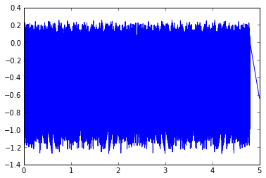
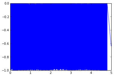
It looks like noise, except for the portion where the velocity is near zero (but not exactly zero). Also, the noise is about 1.4 counts in magnitude peak-to-peak: a perfect encoder would show a peak-to-peak quantization error of 1.0 counts in magnitude, whereas the imperfect encoder adds some error. Let's look at the perfect encoder:
encPerfect = PerfectEncoder(256)
perfectEncoderMeasuredPos = encPerfect.measure(theta_m)
plt.plot(t,actualPosInCounts - perfectEncoderMeasuredPos)
[]
Now all we need is a test algorithm, and a test harness. For an estimation algorithm, let's just take differences of position samples, and put them through a low-pass filter.
class SimpleEstimator(object):
    def __init__(self, lpfcoeff):
        self.velstate = 0
        self.prevpos = 0
        self.lpfcoeff = lpfcoeff
    def usesEdgeTimes(self):
        '''Returns True or False:
           True if the estimator uses edge times, False if it does not.'''
        return False
    def onEdge(self, timeticks, count):
        '''Called at each edge;
        timeticks is an integer in 10-nanosecond ticks
        count is an integer. No return value is necessary.'''
        pass
    def estimatePosVel(self, timetocks, count):
        '''Called at a 10kHz rate.
        timetocks is an integer in 100-microsecond tocks
        count is an integer.
        You should return a 2-element tuple containing a position and velocity
        estimate. Both position and velocity may be scaled to units of your choice.'''
        deltaCount = count - self.prevpos
        self.prevpos = count
        newVelocityEstimate = self.velstate + self.lpfcoeff * (
                                deltaCount - self.velstate)
        self.velstate = newVelocityEstimate
        return (count, newVelocityEstimate)
    def getPosVelScalingFactors(self):
        '''You should return a 2-element tuple (posU, velU) containing
        position and velocity scaling factors. The results of estimatePosVel() are
        interpreted using these scaling factors: the product (position*posU)
        should be measured in mechanical revolutions, and the product (velocity*velU)
        should be measured in mechanical revolutions per second.'''
        return (1.0/256, 1.0/256/100e-6)

import time

def testEstimator(estimator, t, omega_m, theta_m):
    enc = LuckyWheelEncoderUnit1()
    quantizedPosition = enc.measure(theta_m)
    tposlist = zip(t/100e-6, quantizedPosition)

    tstart = time.time()
    # here's where the estimator actually does stuff
    pvlist = [estimator.estimatePosVel(t, pos) for (t,pos) in tposlist]
    tend = time.time()

    (posest_unscaled,velest_unscaled) = zip(*pvlist)
    # unzip the pos + velocity estimates
    (posfactor, velfactor) = estimator.getPosVelScalingFactors()
    return (tend-tstart, np.array(posest_unscaled)*posfactor,
            np.array(velest_unscaled)*velfactor)

def runTest(estimator, whichplots=('error')):
    (compute_time, posest, velest) = testEstimator(est1, t, omega_m, theta_m)
    if 'velocity' in whichplots:
        plt.figure();
        plt.plot(t,omega_m,t,velest);
        plt.ylabel('velocity (rev/sec)')
    if 'error' in whichplots:
        plt.figure();
        plt.plot(t,omega_m-velest);
        plt.ylabel('velocity error (rev/sec)')
    print "This estimator took %.3f msec" % (compute_time*1000)

est1 = SimpleEstimator(0.02)
runTest(est1,('velocity','error'))
This estimator took 869.762 msec
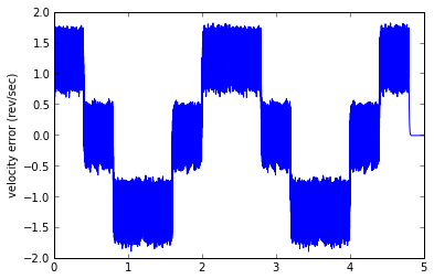
Woot woot! This simple estimator and test harness took me about 15 minutes to code up in Python, and it WORKS!
Except... well, let's get some perspective for the error. An error of 2 revolutions per second is 120RPM, which is kind of high for a velocity error. We have two components of error. One component is the "noise" band, which looks to be about 0.8 rev/sec (around 50RPM) peak-to-peak. This is caused by the encoder quantization error. The other component is an offset proportional to acceleration: this is due to the phase lag caused by the low-pass filter.
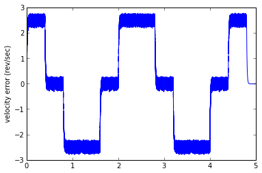
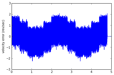
And here we see a dilemma, which will lead nicely into Part II. With a smaller low-pass filter coefficient (lower cutoff frequency), you can reduce the noise band, but the phase lag increases, and the offset proportional to acceleration increases. With a larger low-pass filter coefficient (higher cutoff frequency), you can reduce the offset proportional to acceleration, but the noise band increases. Don't believe me? Let's try it:
est1 = SimpleEstimator(0.01)
runTest(est1)
This estimator took 904.040 msec
est1 = SimpleEstimator(0.05)
runTest(est1)
This estimator took 835.717 msec
Performance Metrics
Finally, we need to talk at least a little about computing a performance metric. The mean squared error is a good one, but we should be a little careful about what constitutes a good estimate of velocity, since different consumers of velocity estimates will be more or less sensitive to different types of error.
Let's consider a velocity control loop; it's going to have a certain transfer function to output velocity and to torque (or current) command. The high-frequency components of speed measurement error have almost no effect on output velocity; the low-frequency components do. Also we don't really care about individual spikes of error, because they'll get filtered out by the system inertia. If we look at the torque command output of the controller, however, high-frequency noise will get multiplied by a speed loop's proportional term, and will create audible noise in a motor. More seriously, large spikes in current command can cause problems in a current controller. So we care about both high frequency and low frequency components, and we care both about large spikes and mean squared error.
The same kinds of things hold true for a current loop that uses speed as a feedforward input, but here we probably don't care too much about low-frequency error, it's the high-frequency error and the current spikes.
I'll talk more in detail about performance metrics in a future column, but for now just keep it in mind that a visual check of the velocity error waveform isn't enough; we really need a quantitative way to compare the results of different estimators.
I hope this has given you a better idea of what it takes to evaluate a particular estimator. Stay tuned for more information on encoder estimation, and on the contest.
© 2013 Jason M. Sachs, all rights reserved.
Stay tuned for a link to this code in an IPython Notebook. I'll put it up on the web, and I do plan to release this in an open-source license, I just have to do a little more homework before I pick the right one.


- Comments
- Write a Comment Select to add a comment
If you would allow plain C code, I would probably send in a decent entry; if you insist on python, I most likely won't participate.

Out of interest, what precise scenario is motivating you to limit what Python entrants can import or invoke? If I were proposing such a contest, my first instinct would be to let people use whatever code they like (incl. 3rd party libraries, so long as they are clearly specified in a requirements.txt and 'pip install' without hassle on my part.)
I can imagine some entries might not run quickly enough, or might produce incorrect results - these would be score poorly the competition. Some code might even hang interminably - yielding a zero score, presumably. But I can't imagine you're really going to get 'bad actor' entrants who attempt to do something malicious when you run their code. Is that what you're guarding against?
I haven't done anything like this since Electronics undergrad (been other types of software ever since) so I'm a total layman at this, forgive me if the answers ought to be obvious
To post reply to a comment, click on the 'reply' button attached to each comment. To post a new comment (not a reply to a comment) check out the 'Write a Comment' tab at the top of the comments.
Please login (on the right) if you already have an account on this platform.
Otherwise, please use this form to register (free) an join one of the largest online community for Electrical/Embedded/DSP/FPGA/ML engineers: