Shibboleths: The Perils of Voiceless Sibilant Fricatives, Idiot Lights, and Other Binary-Outcome Tests
AS-SALT, JORDAN — Dr. Reza Al-Faisal once had a job offer from Google to work on cutting-edge voice recognition projects. He turned it down. The 37-year-old Stanford-trained professor of engineering at Al-Balqa’ Applied University now leads a small cadre of graduate students in a government-sponsored program to keep Jordanian society secure from what has now become an overwhelming influx of refugees from the Palestinian-controlled West Bank. “Sometimes they visit relatives here in Jordan and try to stay here illegally,” he says. “We already have our own unemployment problems, especially among the younger generation.”
Al-Faisal’s group has come up with a technological solution, utilizing drones and voice recognition. “The voice is the key. Native Arabic speakers in West Bank and East Bank populations have noticeable differences in their use of voiceless sibilant fricatives.” He points to a quadcopter drone, its four propellers whirring as it hovers in place. “We have installed a high-quality audio system onto these drones, with a speaker and directional microphones. The drone is autonomous. It presents a verbal challenge to the suspect. When the suspect answers, digital signal processing computes the coefficient of palatalization. East Bank natives have a mean palatalization coefficient of 0.85. With West Bank natives it is only 0.59. If the coefficient is below the acceptable threshold, the drone immobilizes the suspect with nonlethal methods until the nearest patrol arrives.”
One of Al-Faisal’s students presses a button and the drone zooms up and off to the west, embarking on another pilot run. If Al-Faisal’s system, the SIBFRIC-2000, proves to be successful in these test runs, it is likely to be used on a larger scale — so that limited Jordanian resources can cover a wider area to patrol for illegal immigrants. “Two weeks ago we caught a group of eighteen illegals with SIBFRIC. Border Security would never have found them. It’s not like in America, where you can discriminate against people because they look different. East Bank, West Bank — we all look the same. We sound different. I am confident the program will work.”
But some residents of the region are skeptical. “My brother was hit by a drone stunner on one of these tests,” says a 25-year old bus driver, who did not want his name to be used for this story. “They said his voice was wrong. Our family has lived in Jordan for generations. We are proud citizens! How can you trust a machine?”
Al-Faisal declines to give out statistics on how many cases like this have occurred, citing national security concerns. “The problem is being overstated. Very few of these incidents have occurred, and in each case the suspect is unharmed. It does not take long for Border Security to verify citizenship once they arrive.”
Others say there are rumors of voice coaches in Nablus and Ramallah, helping desperate refugees to beat the system. Al-Faisal is undeterred. “Ha ha ha, this is nonsense. SIBFRIC has a perfect ear; it can hear the slightest nuances of speech. You cannot cheat the computer.”
When asked how many drones are in the pilot program, Al-Faisal demures. “More than five,” he says, “fewer than five hundred.” Al-Faisal hopes to ramp up the drone program starting in 2021.
Shame Old Shtory, Shame Old Shong and Dansh
Does this story sound familiar? It might. Here’s a similar one from several thousand years earlier:
5 And the Gileadites took the passages of Jordan before the Ephraimites: and it was so, that when those Ephraimites which were escaped said, Let me go over; that the men of Gilead said unto him, Art thou an Ephraimite? If he said, Nay; 6 Then said they unto him, Say now Shibboleth: and he said Sibboleth: for he could not frame to pronounce it right. Then they took him, and slew him at the passages of Jordan: and there fell at that time of the Ephraimites forty and two thousand.
This is the reputed biblical origin of the term shibboleth, which has come to mean any distinguishing cultural behavior that can be used to identify a particular group, not just a linguistic one. The Ephraimites couldn’t say SHHHH and it became a dead giveaway of their origin.
In this article, we’re going to talk about the shibboleth and several other diagnostic tests which have one of two outcomes — pass or fail, yes or no, positive or negative — and some of the implications of using such a test. And yes, this does impact embedded systems. We’re going to spend quite a bit of time looking at a specific example in mathematical terms. If you don’t like math, just skip it whenever it gets too “mathy”.
A quantitative shibboleth detector
So let’s say we did want to develop a technological test for separating out people who couldn’t say SHHH, and we had some miracle algorithm to evaluate a “palatalization coefficient” \( P_{SH} \) for voiceless sibilant fricatives. How would we pick the threshold?
Well, the first thing to do is try to model the system somehow. We took a similar approach in an earlier article on design margin, where our friend the Oracle computed probability distributions for boiler pressures. Let’s do the same here. Suppose the Palestinians (which we’ll call Group 1) have a \( P_{SH} \) which roughly follows a Gaussian distribution with mean μ = 0.59 and standard deviation σ = 0.06, and the Jordanians (which we’ll call Group 2) have a \( P_{SH} \) which is also a Gaussian distribution with a mean μ = 0.85 and a standard deviation σ = 0.03.
import numpy as np
import matplotlib.pyplot as plt
%matplotlib inline
import scipy.stats
from collections import namedtuple

class Gaussian1D(namedtuple('Gaussian1D','mu sigma name id color')):
    """ Normal (Gaussian) distribution of one variable """
    def pdf(self, x):
        """ probabiliy density function """
        return scipy.stats.norm.pdf(x, self.mu, self.sigma)
    def cdf(self, x):
        """ cumulative distribution function """
        return scipy.stats.norm.cdf(x, self.mu, self.sigma)

d1 = Gaussian1D(0.59, 0.06, 'Group 1 (Palestinian)','P','red')
d2 = Gaussian1D(0.85, 0.03, 'Group 2 (Jordanian)','J','blue')

def show_binary_pdf(d1, d2, x, fig=None, xlabel=None):
    if fig is None:
        fig = plt.figure(figsize=(6,3))
    ax=fig.add_subplot(1,1,1)

    for d in (d1,d2):
        ax.plot(x,d.pdf(x),label=d.name,color=d.color)

    ax.legend(loc='best',labelspacing=0,fontsize=11)
    if xlabel is not None:
        ax.set_xlabel(xlabel, fontsize=15)
    ax.set_ylabel('probability density')
    return ax

show_binary_pdf(d1,d2,x=np.arange(0,1,0.001), xlabel='$P_{SH}$');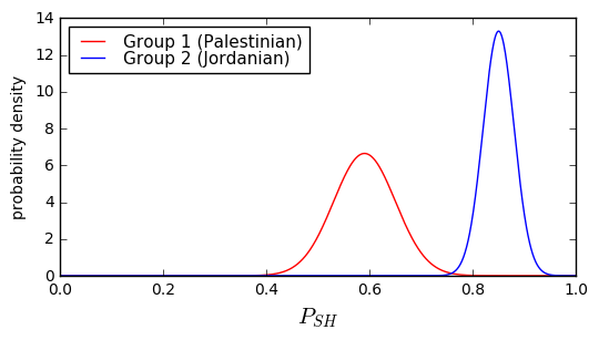
Hmm, we have a dilemma here. Both groups have a small possibility that the \( P_{SH} \) measurement is in the 0.75-0.8 range, and this makes it harder to distinguish. Suppose we decided to set the threshold at 0.75. What would be the probability of our conclusion being wrong?
for d in (d1,d2):
    print '%-25s %f' % (d.name, d.cdf(0.75))
Group 1 (Palestinian) 0.996170 Group 2 (Jordanian) 0.000429
Here the cdf method calls the scipy.stats.norm.cdf function to compute the cumulative distribution function, which is the probability that a given sample from the distribution will be less than a given amount. So there’s a 99.617% chance that Group 1’s \( P_{SH} < 0.75 \), and a 0.0429% chance that Group 2’s \( P_{SH} < 0.75 \). One out of every 261 samples from Group 1 will pass the test (though we were hoping for them to fail) — this is known as a false negative, because a condition that exists (\( P_{SH} < 0.75 \)) remains undetected. One out of every 2331 samples from Group 2 will fail the test (though we were hoping for them to pass) — this is known as a false positive, because a condition that does not exist (\( P_{SH} < 0.75 \)) is mistakenly detected.
The probabilities of false positive and false negative are dependent on the threshold:
for threshold in [0.72,0.73,0.74,0.75,0.76,0.77,0.78]:
    c = [d.cdf(threshold) for d in (d1,d2)]
    print("threshold=%.2f, Group 1 false negative=%7.5f%%, Group 2 false positive=%7.5f%%"
          % (threshold, 1-c[0], c[1]))

threshold = np.arange(0.7,0.801,0.005)
false_positive = d2.cdf(threshold)
false_negative = 1-d1.cdf(threshold)
figure = plt.figure()
ax = figure.add_subplot(1,1,1)
ax.semilogy(threshold, false_positive, label='false positive', color='red')
ax.semilogy(threshold, false_negative, label='false negative', color='blue')
ax.set_ylabel('Probability')
ax.set_xlabel('Threshold $P_{SH}$')
ax.legend(labelspacing=0,loc='lower right')
ax.grid(True)
ax.set_xlim(0.7,0.8);
threshold=0.72, Group 1 false negative=0.01513%, Group 2 false positive=0.00001% threshold=0.73, Group 1 false negative=0.00982%, Group 2 false positive=0.00003% threshold=0.74, Group 1 false negative=0.00621%, Group 2 false positive=0.00012% threshold=0.75, Group 1 false negative=0.00383%, Group 2 false positive=0.00043% threshold=0.76, Group 1 false negative=0.00230%, Group 2 false positive=0.00135% threshold=0.77, Group 1 false negative=0.00135%, Group 2 false positive=0.00383% threshold=0.78, Group 1 false negative=0.00077%, Group 2 false positive=0.00982%

If we want a lower probability of false positives (fewer Jordanians detained for failing the test) we can do so by lowering the threshold, but at the expense of raising the probability of false negatives (more Palestinians unexpectedly passing the test and not detained), and vice-versa.
Factors used in choosing a threshold
There is a whole science around binary-outcome tests, primarily in the medical industry, involving sensivity and specificity, and it’s not just a matter of probability distributions. There are two other aspects that make a huge difference in determining a good test threshold:
- base rate — the probability of the condition actually being true, sometimes referred as prevalence in medical diagnosis
- the consequences of false positives and false negatives
Both of these are important because they affect our interpretation of false positive and false negative probabilities.
Base rate
The probabilities we calculated above are conditional probabilities — in our example, we calculated the probability that a person known to be from the Palestinian population passed the SIBFRIC test, and the probability that a person known to be from the Jordanian population failed the SIBFRIC tests.
It’s also important to consider the joint probability distribution — suppose that we are trying to detect a very uncommon condition. In this case the false positive rate will be amplified relative to the false negative rate. Let’s say we have some condition C that has a base rate of 0.001, or one in a thousand, and there is a test with a false positive rate of 0.2% and a false negative rate of 5%. This sounds like a really bad test: we should balance the probabilities by lowering the false negative rate and allowing a higher false positive rate. The net incidence of false positives for C will be 0.999 × 0.002 = 0.001998, and the net incidence of false negatives will be 0.001 × 0.05 = 0.00005. If we had one million people we test for condition C:
- 1000 actually have condition C
- 950 people are correctly diagnosed has having C
- 50 people will remain undetected (false negatives)
- 999000 do not actually have condition C
- 997002 people are correctly diagnosed as not having C
- 1998 people are incorrectly diagnosed as having C (false positives)
The net false positive rate is much higher than the net false negative rate, and if we had a different test with a false positive rate of 0.1% and a false negative rate of 8%, this might actually be better, even though the conditional probabilities of false positives and false negatives look even more lopsided. This is known as the false positive paradox.
Consequences
Let’s continue with our hypothetical condition C with a base rate of 0.001, and the test that has a false positive rate of 0.2% and a false negative rate of 5%. And suppose that the consequences of false positives are unnecessary hospitalization and the consequences of false negatives are certain death:
- 997002 diagnosed as not having C → relief
- 1998 incorrectly diagnosed as having C → unnecessary hospitalization, financial cost, annoyance
- 950 correctly diagnosed as having C → treatment, relief
- 50 incorrectly diagnosed as not having C → death
If the test can be changed, we might want to reduce the false negative, even if it raises the net false positive rate higher. Would lowering 50 deaths per million to 10 deaths per million be worth it if it raises the false positive rate of unnecessary hospitalization from 1998 per million to, say, 5000 per million? 20000 per million?
Consequences can rarely be compared directly; more often we have an apples-to-oranges comparison like death vs. unnecessary hospitalization, or allowing criminals to be free vs. incarcerating the innocent. If we want to handle a tradeof quantitatively, we’d need to assign some kind of metric for the consequences, like assigning a value of \$10 million for an unnecessary death vs. \$10,000 for an unnecessary hospitalization — in such a case we can minimize the net expected loss over an entire population. Otherwise it becomes an ethical question. In jurisprudence there is the idea of Blackstone’s ratio: “It is better that ten guilty persons escape than that one innocent suffer.” But the post-2001 political climate in the United States seems to be that detaining the innocent is more desirable than allowing terrorists or illegal immigrants to remain at large. Mathematics alone won’t help us out of these quandaries.
Optimizing a threshold
OK, so suppose we have a situation that can be described completely in mathematical terms:
- \( A \): Population A can be measured with parameter \( x \) with probability density function \( f_A(x) \) and cumulative density function \( F_A(x) = \int\limits_{-\infty}^x f_A(u) \, du \)
- \( B \): Population B can be measured with parameter \( x \) with PDF \( f_B(x) \) and CDF \( F_B(x) = \int\limits_{-\infty}^x f_B(u) \, du \)
- All samples are either in \( A \) or \( B \):
- \( A \) and \( B \) are disjoint (\( A \cap B = \varnothing \))
- \( A \) and \( B \) are collectively exhaustive (\( A \cup B = \Omega \), where \( \Omega \) is the full sample space, so that \( P(A \ {\rm or}\ B) = 1 \))
- Some threshold \( x_0 \) is determined
- For any given sample \( s \) that is in either A or B (\( s \in A \) or \( s \in B \), respectively), parameter \( x_s \) is compared with \( x_0 \) to determine an estimated classification \( a \) or \( b \):
- \( a \): if \( x_s > x_0 \) then \( s \) is likely to be in population A
- \( b \): if \( x_s \le x_0 \) then \( s \) is likely to be in population B
- Probability of \( s \in A \) is \( p_A \)
- Probability of \( s \in B \) is \( p_B = 1-p_A \)
- Value of various outcomes:
- \( v_{Aa} \): \( s \in A, x_s > x_0 \), correctly classified in A
- \( v_{Ab} \): \( s \in A, x_s \le x_0 \), incorrectly classified in B
- \( v_{Ba} \): \( s \in B, x_s > x_0 \), incorrectly classified in A
- \( v_{Bb} \): \( s \in B, x_s \le x_0 \), correctly classified in B
The expected value over all outcomes is
$$\begin{aligned} E[v] &= v_{Aa}P(Aa)+v_{Ab}P(Ab) + v_{Ba}P(Ba) + v_{Bb}P(Bb)\cr &= v_{Aa}p_A P(a\ |\ A) \cr &+ v_{Ab}p_A P(b\ |\ A) \cr &+ v_{Ba}p_B P(a\ |\ B) \cr &+ v_{Bb}p_B P(b\ |\ B) \end{aligned}$$
These conditional probabilities \( P(a\ |\ A) \) (denoting the probability of the classification \( a \) given that the sample is in \( A \)) can be determined with the CDF functions; for example, if the sample is in A then \( P(a\ |\ A) = P(x > x_0\ |\ A) = 1 - P(x \le x_0) = 1 - F_A(x_0) \), and once we know that, then we have
$$\begin{aligned} E[v] &= v_{Aa}p_A (1-F_A(x_0)) \cr &+ v_{Ab}p_A F_A(x_0) \cr &+ v_{Ba}p_B (1-F_B(x_0)) \cr &+ v_{Bb}p_B F_B(x_0) \cr E[v] &= p_A \left(v_{Ab} + (v_{Aa}-v_{Ab})\left(1-F_A(x_0)\right)\right) \cr &+ p_B \left(v_{Bb} + (v_{Ba}-v_{Bb})\left(1-F_B(x_0)\right)\right) \end{aligned}$$
\( E[v] \) is actually a function of the threshold \( x_0 \), and we can locate its maximum value by determining points where its partial derivative \( {\partial E[v] \over \partial {x_0}} = 0: \)
$$0 = {\partial E[v] \over \partial {x_0}} = p_A(v_{Ab}-v_{Aa})f_A(x_0) + p_B(v_{Bb}-v_{Ba})f_B(x_0)$$
$${f_A(x_0) \over f_B(x_0)} = \rho_p \rho_v = -\frac{p_B(v_{Bb}-v_{Ba})}{p_A(v_{Ab}-v_{Aa})}$$
where the \( \rho \) are ratios for probability and for value tradeoffs:
$$\begin{aligned} \rho_p &= p_B/p_A \cr \rho_v &= -\frac{v_{Bb}-v_{Ba}}{v_{Ab}-v_{Aa}} \end{aligned}$$
One interesting thing about this equation is that since probabilities \( p_A \) and \( p_B \) and PDFs \( f_A \) and \( f_B \) are positive, this means that \( v_{Bb}-v_{Ba} \) and \( v_{Ab}-v_{Aa} \) must be opposite signs, otherwise… well, let’s see:
Case study: Embolary Pulmonism
Suppose we have an obscure medical condition; let’s call it an embolary pulmonism, or EP for short. This must be treated within 48 hours, or the patient can transition in minutes from seeming perfectly normal, to a condition in which a small portion of their lungs degrade rapidly, dissolve, and clog up blood vessels elsewhere in the body, leading to extreme discomfort and an almost certain death. Before this rapid decline, the only symptoms are a sore throat and achy eyes.
We’re developing an inexpensive diagnostic test \( T_1 \) (let’s suppose it costs \$1) where the patient looks into a machine and it takes a picture of the patient’s eyeballs and uses machine vision to come up with some metric \( x \) that can vary from 0 to 100. We need to pick a threshold \( x_0 \) such that if \( x > x_0 \) we diagnose the patient with EP.
Let’s consider some math that’s not quite realistic:
- condition A: patient has EP
- condition B: patient does not have EP
- incidence of EP in patients complaining of sore throats and achy eyes: \( p_A = \) 0.004% (40 per million)
- value of Aa (correct diagnosis of EP): \( v_{Aa}=- \) \$100000
- value of Ab (false negative, patient has EP, diagnosis of no EP): \( v_{Ab}=0 \)
- value of Ba (false positive, patient does not have EP, diagnosis of EP): \( v_{Ba}=- \)\$5000
- value of Bb (correct diagnosis of no EP): \( v_{Bb} = 0 \)
So we have \( v_{Ab}-v_{Aa} = \) \$100000 and \( v_{Bb}-v_{Ba} = \) \$5000, for a \( \rho_v = -0.05, \) which implies that we’re looking for a threshold \( x_0 \) where \( \frac{f_A(x_0)}{f_B(x_0)} = -0.05\frac{p_B}{p_A} \) is negative, and that never occurs with any real probability distributions. In fact, if we look carefully at the values \( v \), we’ll see that when we diagnose a patient with EP, it always has a higher cost: If we correctly diagnose them with EP, it costs \$100,000 to treat. If we incorrectly diagnose them with EP, it costs \$5,000, perhaps because we can run a lung biopsy and some other fancy test to determine that it’s not EP. Whereas if we give them a negative diagnosis, it doesn’t cost anything. This implies that we should always prefer to give patients a negative diagnosis. So we don’t even need to test them!
Patient: “Hi, Doc, I have achy eyes and a sore throat, do I have EP?”
Doctor: (looks at patient’s elbows studiously for a few seconds) “Nope!”
Patient: (relieved) “Okay, thanks!”
What’s wrong with this picture? Well, all the values look reasonable except for two things. First, we haven’t included the \$1 cost of the eyeball test… but that will affect all four outcomes, so let’s just state that the values \( v \) are in addition to the cost of the test. The more important issue is the false negative, the Ab case, where the patient is diagnosed incorrectly as not having EP, and it’s likely the patient will die. Perhaps the hospital’s insurance company has estimated a cost of \$10 million per case to cover wrongful death civil suits, in which case we should be using \( v _ {Ab} = -\$10^7 \). So here’s our revised description:
- condition A: patient has EP
- condition B: patient does not have EP
- incidence of EP in patients complaining of sore throats and achy eyes: \( p_A = \) 0.004% (40 per million)
- value of Aa (correct diagnosis of EP): \( v_{Aa}=- \) \$100000 (rationale: mean cost of treatment)
- value of Ab (false negative, patient has EP, diagnosis of no EP): \( v_{Ab}=-\$10^7 \) (rationale: mean cost of resulting liability due to high risk of death)
- value of Ba (false positive, patient does not have EP, diagnosis of EP): \( v_{Ba}=- \)\$5000 (rationale: mean cost of additional tests to confirm)
- value of Bb (correct diagnosis of no EP): \( v_{Bb} = 0 \) (rationale: no further treatment needed)
The equation for choosing \( x_0 \) then becomes
$$\begin{aligned} \rho_p &= p_B/p_A = 0.99996 / 0.00004 = 24999 \cr \rho_v &= -\frac{v_{Bb}-v_{Ba}}{v_{Ab}-v_{Aa}} = -5000 / {-9.9}\times 10^6 \approx 0.00050505 \cr {f_A(x_0) \over f_B(x_0)} &= \rho_p\rho_v \approx 12.6258. \end{aligned}$$
Now we need to know more about our test. Suppose that the results of the eye machine test have normal probability distributions with \( \mu=55, \sigma=5.3 \) for patients with EP and \( \mu=40, \sigma=5.9 \) for patients without EP.
x = np.arange(0,100,0.1)
dpos = Gaussian1D(55, 5.3, 'A (EP-positive)','A','red')
dneg = Gaussian1D(40, 5.9, 'B (EP-negative)','B','green')

show_binary_pdf(dpos, dneg, x, xlabel = 'test result $x$');
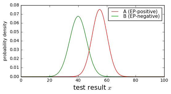
Yuck. This doesn’t look like a very good test; there’s a lot of overlap between the probability distributions.
At any rate, suppose we pick a threshold \( x_0=47 \); what kind of false positive / false negative rates will we get, and what’s the expected overall value?
import IPython.core.display
from IPython.display import display, HTML

def analyze_binary(dneg, dpos, threshold):
    """
    Returns confusion matrix
    """
    pneg = dneg.cdf(threshold)
    ppos = dpos.cdf(threshold)
    return np.array([[pneg, 1-pneg],
                     [ppos, 1-ppos]])

def show_binary_matrix(confusion_matrix, threshold, distributions,
                       outcome_ids, ppos, vmatrix,
                       special_format=None):
    if special_format is None:
        special_format = {}
    def cellinfo(c, p, v):
        # joint probability = c*p
        jp = c*p
        return (c, jp, jp*v)
    def rowcalc(i,confusion_row):
        """ write this for rows containing N elements, not just 2 """
        p = ppos if (i == 1) else (1-ppos)
        return [cellinfo(c,p,vmatrix[i][j]) for j,c in enumerate(confusion_row)]
    Jfmtlist = special_format.get('J')
    cfmtlist = special_format.get('c')
    vfmtlist = special_format.get('v')
    try:
        if isinstance(vfmtlist, basestring):
            vfmt_general = vfmtlist
        else:
            vfmt_general = vfmtlist[0]
    except:
        vfmt_general = '%.3f'
    def rowfmt(row,dist):
        def get_format(fmt, icell, default):
            if fmt is None:
                return default
            if isinstance(fmt,basestring):
                return fmt
            return fmt[icell] or default
        def cellfmt(icell):
            Jfmt = get_format(Jfmtlist, icell, '%.7f')
            cfmt = get_format(cfmtlist, icell, '%.5f')
            vfmt = get_format(vfmtlist, icell, '%.3f')
            return '<td>'+cfmt+'<br>J='+Jfmt+'<br>wv='+vfmt+'</td>'
        return '<th>'+dist.name+'</th>' + ''.join(
                  (cellfmt(i) % cell)
                  for i,cell in enumerate(row))

    rows = [rowcalc(i,row) for i,row in enumerate(confusion_matrix)]
    vtot = sum(v for row in rows for c,J,v in row)
    if not isinstance (threshold, basestring):
        threshold = 'x_0 = %s' % threshold

    return HTML(('<p>Report for threshold \\(%s \\rightarrow E[v]=\\)'
                 +vfmt_general+'</p>')%(threshold,vtot)
                +'<table><tr><td></td>'+
                ''.join('<th>%s</th>' % id for id in outcome_ids)
                +'</tr>'
                +''.join('<tr>%s</tr>' % rowfmt(row,dist)
                         for row,dist in zip(rows,distributions))
                +'</table>')

threshold = 47
C = analyze_binary(dneg, dpos, threshold)
show_binary_matrix(C, threshold, [dneg, dpos], 'ba', 40e-6,[[0,-5000],[-1e7, -1e5]],
                   special_format={'v':'$%.2f'})
Report for threshold \(x_0 = 47 \rightarrow E[v]=\)$-618.57
| b | a | |
|---|---|---|
| B (EP-negative) | 0.88228 J=0.8822406 wv=$0.00 | 0.11772 J=0.1177194 wv=$-588.60 |
| A (EP-positive) | 0.06559 J=0.0000026 wv=$-26.24 | 0.93441 J=0.0000374 wv=$-3.74 |
Here we’ve shown a modified confusion matrix showing for each of the four outcomes the following quantities:
- Conditional probability of each outcome: \( \begin{bmatrix}P(b\ |\ B) & P(a\ |\ B) \cr P(b\ |\ A) & P(a\ |\ A)\end{bmatrix} \) — read each entry like \( P(a\ |\ B) \) as “the probability of \( a \), given that \( B \) is true”, so that the numbers in each row add up to 1
- J: Joint probability of the outcome: \( \begin{bmatrix}P(Bb) & P(Ba) \cr P(Ab) & P(Aa)\end{bmatrix} \) — read each entry like \( P(Ba) \) as “The probability that \( B \) and \( a \) are true”, so that the numbers in the entire matrix add up to 1
- wv: Weighted contribution to expected value = joint probability of the outcome × its value
For example, if the patient does not have EP, there’s about an 88.2% chance that they will be diagnosed correctly and an 11.8% chance that the test will produce a false positive. If the patient does have EP, there’s about a 6.6% chance the test will produce a false negative, and a 93.4% chance the test will correctly diagnose that they have EP.
The really interesting thing here is the contribution to expected value. Remember, the false negative (Ab) is really bad, since it has a value of \$10 million, but it’s also very rare because of the low incidence of EP and the fact that condtional probability of a false negative is only 6.6%. Whereas the major contribution to expected value comes from the false positive case (Ba) that occurs in almost 11.8% of the population.
We should be able to use a higher threshold to reduce the expected cost over the population:
for threshold in [50, 55]:
    C = analyze_binary(dneg, dpos, threshold)
    display(show_binary_matrix(C, threshold, [dneg, dpos], 'ba', 40e-6,[[0,-5000],[-1e7, -1e5]],
                               special_format={'v':'$%.2f'}))
Report for threshold \(x_0 = 50 \rightarrow E[v]=\)$-297.62
| b | a | |
|---|---|---|
| B (EP-negative) | 0.95495 J=0.9549161 wv=$0.00 | 0.04505 J=0.0450439 wv=$-225.22 |
| A (EP-positive) | 0.17274 J=0.0000069 wv=$-69.10 | 0.82726 J=0.0000331 wv=$-3.31 |
Report for threshold \(x_0 = 55 \rightarrow E[v]=\)$-229.52
| b | a | |
|---|---|---|
| B (EP-negative) | 0.99449 J=0.9944551 wv=$0.00 | 0.00551 J=0.0055049 wv=$-27.52 |
| A (EP-positive) | 0.50000 J=0.0000200 wv=$-200.00 | 0.50000 J=0.0000200 wv=$-2.00 |
The optimal threshold should probably be somewhere between \( x_0=50 \) and \( x_0=55 \), since in one case the contributions to expected value is mostly from the false positive case, and in the other from the false negative case. If we have a good threshold, these contributions are around the same order of magnitude from the false positive and false negative cases. (They won’t necessarily be equal, though.)
To compute this threshold we are looking for
$$\rho = {f_A(x_0) \over f_B(x_0)} = \rho_p\rho_v \approx 12.6258.$$
We can either solve it using numerical methods, or try to solve analytically using the normal distribution probability density
$$f(x) = \frac{1}{\sigma\sqrt{2\pi}}e^{-(x-\mu)^2/2\sigma^2}$$
which gives us
$$\frac{1}{\sigma_A}e^{-(x_0-\mu_A)^2/2\sigma_A{}^2} = \frac{1}{\sigma_B}\rho e^{-(x_0-\mu_B)^2/2\sigma_B{}^2}$$
and taking logs, we get
$$-\ln\sigma_A-(x_0-\mu_A)^2/2\sigma_A{}^2 = \ln\rho -\ln\sigma_B-(x_0-\mu_B)^2/2\sigma_B{}^2$$
If we set \( u = x_0 - \mu_A \) and \( \Delta = \mu_B - \mu_A \) then we get
$$-u^2/2\sigma_A{}^2 = \ln\rho\frac{\sigma_A}{\sigma_B} -(u-\Delta)^2/2\sigma_B{}^2$$
$$-\sigma_B{}^2u^2 = 2\sigma_A{}^2\sigma_B{}^2\left(\ln\rho\frac{\sigma_A}{\sigma_B} \right) -\sigma_A{}^2(u^2 - 2\Delta u + \Delta^2)$$
which simplifies to \( Au^2 + Bu + C = 0 \) with
$$\begin{aligned} A &= \sigma_B{}^2 - \sigma_A{}^2 \cr B &= 2\Delta\sigma_A{}^2 \cr C &= 2\sigma_A{}^2\sigma_B{}^2\left(\ln\rho\frac{\sigma_A}{\sigma_B}\right) - \Delta^2\sigma_A{}^2 \end{aligned}$$
We can solve this with the alternate form of the quadratic formula \( u = \frac{2C}{-B \pm \sqrt{B^2-4AC}} \) which can compute the root(s) even with \( A=0\ (\sigma_A = \sigma_B = \sigma) \), where it simplifies to \( u=-C/B=\frac{-\sigma^2 \ln \rho}{\mu_B - \mu_A} + \frac{\mu_B - \mu_A}{2} \) or \( x_0 = \frac{\mu_B + \mu_A}{2} - \frac{\sigma^2 \ln \rho}{\mu_B - \mu_A} \).
def find_threshold(dneg, dpos, ppos, vmatrix):
    num = -(1-ppos)*(vmatrix[0][0]-vmatrix[0][1])
    den = ppos*(vmatrix[1][0]-vmatrix[1][1])
    rho = num/den
    A = dneg.sigma**2 - dpos.sigma**2
    ofs = dpos.mu
    delta = dneg.mu - dpos.mu
    B = 2.0*delta*dpos.sigma**2
    C = (2.0 * dneg.sigma**2 * dpos.sigma**2 * np.log(rho*dpos.sigma/dneg.sigma)
         - delta**2 * dpos.sigma**2)
    if (A == 0):
        roots = [ofs-C/B]
    else:
        D = B*B-4*A*C
        roots = [ofs + 2*C/(-B-np.sqrt(D)),
                 ofs + 2*C/(-B+np.sqrt(D))]

    # Calculate expected value, so that if we have more than one root,
    # the caller can determine which is better
    pneg = 1-ppos
    results = []
    for i,root in enumerate(roots):
        cneg = dneg.cdf(root)
        cpos = dpos.cdf(root)
        Ev =  (cneg*pneg*vmatrix[0][0]
              +(1-cneg)*pneg*vmatrix[0][1]
              +cpos*ppos*vmatrix[1][0]
              +(1-cpos)*ppos*vmatrix[1][1])
        results.append((root,Ev))
    return results

find_threshold(dneg, dpos, 40e-6, [[0,-5000],[-1e7, -1e5]])
[(182.23914143860179, -400.00000000000006), (53.162644275683974, -212.51747111423805)]
threshold =53.1626
for x0 in [threshold, threshold-0.1, threshold+0.1]:
    C = analyze_binary(dneg, dpos, x0)
    display(show_binary_matrix(C, x0, [dneg, dpos], 'ba', 40e-6,[[0,-5000],[-1e7, -1e5]],
                               special_format={'v':'$%.2f'}))
Report for threshold \(x_0 = 53.1626 \rightarrow E[v]=\)$-212.52
| b | a | |
|---|---|---|
| B (EP-negative) | 0.98716 J=0.9871183 wv=$0.00 | 0.01284 J=0.0128417 wv=$-64.21 |
| A (EP-positive) | 0.36442 J=0.0000146 wv=$-145.77 | 0.63558 J=0.0000254 wv=$-2.54 |
Report for threshold \(x_0 = 53.0626 \rightarrow E[v]=\)$-212.58
| b | a | |
|---|---|---|
| B (EP-negative) | 0.98659 J=0.9865461 wv=$0.00 | 0.01341 J=0.0134139 wv=$-67.07 |
| A (EP-positive) | 0.35735 J=0.0000143 wv=$-142.94 | 0.64265 J=0.0000257 wv=$-2.57 |
Report for threshold \(x_0 = 53.2626 \rightarrow E[v]=\)$-212.58
| b | a | |
|---|---|---|
| B (EP-negative) | 0.98771 J=0.9876692 wv=$0.00 | 0.01229 J=0.0122908 wv=$-61.45 |
| A (EP-positive) | 0.37153 J=0.0000149 wv=$-148.61 | 0.62847 J=0.0000251 wv=$-2.51 |
So it looks like we’ve found the threshold \( x_0 = 53.0626 \) to maximize expected value of all possible outcomes at \$-212.52. The vast majority (98.72%) of people taking the test don’t incur any cost or trouble beyond that of the test itself.
Still, it’s somewhat unsatisfying to have such a high false negative rate: over 36% of patients who are EP-positive are undetected by our test, and are likely to die. To put this into perspective, consider a million patients who take this test. The expected number of them for each outcome are
- 12842 will be diagnosed with EP but are actually EP-negative (false positive) and require \$5000 in tests to confirm
- 15 will be EP-positive but will not be diagnosed with EP (false negative) and likely to die
- 25 will be EP-positive and correctly diagnosed and incur \$100,000 in treatment
- the rest are EP-negative and correctly diagnosed.
That doesn’t seem fair to those 15 people, just to help reduce the false positive rate.
We could try skewing the test by assigning a value of \$100 million, rather than \$10 million, for the false negative case, because it’s really really bad:
find_threshold(dneg, dpos, 40e-6, [[0,-5000],[-1e8, -1e5]])
[(187.25596232479654, -4000.0000000000005),
 (48.145823389489138, -813.91495238472135)]
threshold = 48.1458
for x0 in [threshold, threshold-0.1, threshold+0.1]:
    C = analyze_binary(dneg, dpos, x0)
    display(show_binary_matrix(C, x0, [dneg, dpos], 'ba', 40e-6,[[0,-5000],[-1e8, -1e5]],
                               special_format={'v':'$%.2f'}))
Report for threshold \(x_0 = 48.1458 \rightarrow E[v]=\)$-813.91
| b | a | |
|---|---|---|
| B (EP-negative) | 0.91631 J=0.9162691 wv=$0.00 | 0.08369 J=0.0836909 wv=$-418.45 |
| A (EP-positive) | 0.09796 J=0.0000039 wv=$-391.85 | 0.90204 J=0.0000361 wv=$-3.61 |
Report for threshold \(x_0 = 48.0458 \rightarrow E[v]=\)$-814.23
| b | a | |
|---|---|---|
| B (EP-negative) | 0.91367 J=0.9136317 wv=$0.00 | 0.08633 J=0.0863283 wv=$-431.64 |
| A (EP-positive) | 0.09474 J=0.0000038 wv=$-378.96 | 0.90526 J=0.0000362 wv=$-3.62 |
Report for threshold \(x_0 = 48.2458 \rightarrow E[v]=\)$-814.23
| b | a | |
|---|---|---|
| B (EP-negative) | 0.91888 J=0.9188456 wv=$0.00 | 0.08112 J=0.0811144 wv=$-405.57 |
| A (EP-positive) | 0.10126 J=0.0000041 wv=$-405.06 | 0.89874 J=0.0000359 wv=$-3.59 |
There, by moving the threshold downward by about 5 points, we’ve reduced the false negative rate to just under 10%, and the false positive rate is just over 8%. The expected value has nearly quadrupled, though, to \$-813.91, mostly because the false positive rate has increased, but also because the cost of a false negative is much higher.
Now, for every million people who take the test, we would expect
- around 83700 will have a false positive
- 36 will be correctly diagnosed with EP
- 4 will incorrectly remain undiagnosed and likely die.
Somehow that doesn’t sound very satisfying either. Can we do any better?
Idiot lights
Let’s put aside our dilemma of choosing a diagnosis threshold, for a few minutes, and talk about idiot lights. This term generally refers to indicator lights on automotive instrument panels, and apparently showed up in print around 1960. A July 1961 article by Phil McCafferty in Popular Science, called Let’s Bring Back the Missing Gauges, states the issue succinctly:
Car makers have you and me figured out for idiots — to the tune of about eight million dollars a year. This is the estimated amount that auto makers save by selling us little blink-out bulbs — known to fervent nonbelievers as “idiot lights” — on five million new cars instead of fitting them out with more meaningful gauges.
Not everything about blink-outs is bad. They do give a conspicuous warning when something is seriously amiss. But they don’t tell enough, or tell it soon enough to be wholly reliable. That car buyers aren’t happy is attested by the fact that gauge makers gleefully sell some quarter of a million accessory instruments a year to people who insist on knowing what’s going on under their hoods.
He goes on to say:
There’s little consolation in being told your engine has overheated after it’s done it. With those wonderful old-time gauges, a climbing needle gave you warning before you got into trouble.
The basic blink-out principle is contrary to all rules of safety. Blink-outs do not “fail safe.” The system operates on the assurance that all is well when the lights are off. If a bulb burns out while you’re traveling, you’ve lost your warning system.
Sure, most indicators remain on momentarily during starting, which makes it possible to check them for burnouts. But this has been known to have problems.
Consider the Midwestern husband who carefully lectured his young wife on the importance of watching gauges, then traded in the old car for a new blink-out model. Anxious to try it out, the wife fired it up the minute it arrived without waiting for her husband to come home. Panicked by three glaring lights, she assumed the worst, threw open the hood, and was met by the smell of new engine paint burning. Without hesitation, she popped off the cap and filled the crank-case to the brim—with water.
The big blink-out gripe is that the lights fail to tell the degree of what is taking place. Most oil-pressure blink-outs turn off at about 10 to 15 pounds’ pressure. Yet this is not nearly enough to lubricate an engine at 70 m.p.h.
The generator blink-out, unlike an ammeter, tells only whether or not the generator is producing current, not how much. You can be heading for a dead battery if you are using more current than the generator is producing. A battery can also be ruined by pouring an excessive charge into it, and over-production can kill a generator. Yet in all cases the generator is working, so the light is off.
The lights hide the secrets that a sinking, climbing, or fluctuating needle can reveal. Because of this, blink-outs are one of the greatest things that ever happened to a shady used-car dealer.
McCafferty seems to have been a bit of a zealot on this topic, publishing a November 1955 article in Popular Science, I Like the Gauges Detroit Left Out, though it doesn’t mention the term “idiot light”. The earliest use of “idiot light” in common media seems to be in the January 1960 issue of Popular Science, covering some automotive accessories like this volt-ammeter kit:
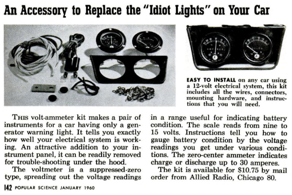
Interestingly enough, on the previous page is an article (TACHOMETER: You Can Assemble One Yourself with This \$14.95 Kit) showing a schematic and installation of a tachometer circuit that gets its input from one of the distributor terminals, and uses a PNP transistor to send a charge pulse to a capacitor and ammeter everytime the car’s distributor sends a high-voltage pulse to the spark plugs:

The earliest use of “idiot light” I could find in any publication is from a 1959 monograph on Standard Cells from the National Bureau of Standards which states
It is realized that the use of good-bad indicators must be approached with caution. Good-bad lights, often disparagingly referred to as idiot lights, are frequently resented by the technician because of the obvious implication. Furthermore, skilled technicians may feel that a good-bad indication does not give them enough information to support their intuitions. However, when all factors are weighed, good-bad indicators appear to best fit the requirements for an indication means that may be interpreted quickly and accurately by a wide variety of personnel whether trained or untrained.
Regardless of the term’s history, we’re stuck with these lights in many cases, and they’re a compromise between two principles:
- idiot lights are an effective and inexpensive method of catching the operator’s attention to one of many possible conditions that can occur, but they hide information by reducing a continuous value to a true/false indication
- a numeric result, shown by a dial-and-needle gauge or a numeric display, can show more useful information than an idiot light, but it is more expensive, doesn’t draw attention as easily as an idiot light, and it requires the operator to interpret the numeric value
¿Por qué no los dos?
If we don’t have an ultra-cost-sensitive system, why not have both? Computerized screens are very common these days, and it’s relatively easy to display both a PASS/FAIL or YES/NO indicator — for drawing attention to a possible problem — and a value that allows the operator to interpret the data.
Since 2008, new cars sold in the United States have been required to have a tire pressure monitoring system (TPMS). As a driver, I both love it and hate it. The TPMS is great for dealing with slow leaks before they become a problem. I carry a small electric tire pump that plugs into the 12V socket in my car, so if the TPMS light comes on, I can pull over, check the tire pressure, and pump up the one that has a leak to its normal range. I’ve had slow leaks that have lasted several weeks before they start getting worse. Or sometimes they’re just low pressure because it’s November or December and the temperature has decreased. What I don’t like is that there’s no numerical gauge. If my TPMS light comes on, I have no way to distinguish a slight decrease in tire pressure (25psi vs. the normal 30psi) vs. a dangerously low pressure (15psi), unless I stop and measure all four tires with a pressure gauge. I have no way to tell how quickly the tire pressure is decreasing, so I can decide whether to keep driving home and deal with it later, or whether to stop at the nearest possible service station. It would be great if my car had an information screen where I could read the tire pressure readings and decide what to do based on having that information.
As far as medical diagnostic tests go, using the extra information from a raw test score can be a more difficult decision, especially in cases where the chances and costs of both false positives and false negatives are high. In the EP example we looked at earlier, we had a 0-to-100 test with a threshold of somewhere in the 55-65 range. Allowing a doctor to use their judgment when interpreting this kind of a test might be a good thing, especially when the doctor can try to make use of other information. But as a patient, how am I to know? If I’m getting tested for EP and I have a 40 reading, my doctor can be very confident that I don’t have EP, whereas with a 75 reading, it’s a no-brainer to start treatment right away. But those numbers near the threshold are tricky.
Triage (¿Por qué no los tres?)
In medicine, the term triage refers to a process of rapid prioritization or categorization in order to determine which patients should be served first. The idea is to try to make the most difference, given limited resources — so patients who are sick or injured, but not in any immediate danger, may have to wait.
As an engineer, my colleagues and I use triage as a way to categorize issues so that we can focus only on the few that are most important. A couple of times a year we’ll go over the unresolved issues in our issue tracking database, to figure out which we’ll address in the near term. One of the things I’ve noticed is that our issues fall into three types:
- Issues which are obviously low priority — these are ones that we can look at in a few seconds and agree, “Oh, yeah, we don’t like that behavior but it’s just a minor annoyance and isn’t going to cause any real trouble.”
- Issues which are obviously high priority — these are ones that we can also look at in a few seconds and agree that we need to address them soon.
- Issues with uncertainty — we look at these and kind of sit and stare for a while, or have arguments within the group, about whether they’re important or not.
The ones in the last category take a lot of time, and slow this process down immensely. I would much rather come to a 30-second consensus of L/H/U (“low priority”/”high priority”/”uncertain”) and get through the whole list, then come back and go through the U issues one by one at a later date.
Let’s go back to our EP case, and use the results of our \$1 eyeball-photography test \( T_1 \), but instead of dividing our diagnosis into two outcomes, let’s divide it into three outcomes:
- Patients are diagnosed as EP-positive, with high confidence
- Patients for which the EP test is “ambivalent” and it is not possible to distinguish between EP-positive and EP-negative cases with high confidence
- Patients are diagnosed as EP-negative, with high confidence
We take the same actions in the EP-positive case (admit patient and begin treatment) and the EP-negative case (discharge patient) as before, but now we have this middle ground. What should we do? Well, we can use resources to evaluate the patient more carefully. Perhaps there’s some kind of blood test \( T_2 \), which costs \$100, but improves our ability to distinguish between EP-positive and EP-negative populations. It’s more expensive than the \$1 test, but much less expensive than the \$5000 run of tests we used in false positive cases in our example.
How can we evaluate test \( T_2 \)?
Bivariate normal distributions
Let’s say that \( T_2 \) also has a numeric result \( y \) from 0 to 100, and it has a Gaussian distribution as well, so that tests \( T_1 \) and \( T_2 \) return a pair of values \( (x,y) \) with a bivariate normal distribution, in particular both \( x \) and \( y \) can be described by their mean values \( \mu_x, \mu_y \), standard deviations \( \sigma_x, \sigma_y \) and correlation coefficient \( \rho \), so that the covariance matrix \( \operatorname{cov}(x,y) = \begin{bmatrix}S_{xx} & S_{xy} \cr S_{xy} & S_{yy}\end{bmatrix} \) can be calculated with \( S_{xx} = \sigma_x{}^2, S_{yy} = \sigma_y{}^2, S_{xy} = \rho\sigma_x\sigma_y. \)
-
When a patient has EP (condition A), the second-order statistics of \( (x,y) \) can be described as
- \( \mu_x = 55, \mu_y = 57 \)
- \( \sigma_x=5.3, \sigma_y=4.1 \)
- \( \rho = 0.91 \)
-
When a patient does not have EP (condition B), the second-order statistics of \( (x,y) \) can be described as
- \( \mu_x = 40, \mu_y = 36 \)
- \( \sigma_x=5.9, \sigma_y=5.2 \)
- \( \rho = 0.84 \)
The covariance matrix may be unfamiliar to you, but it’s not very complicated. (Still, if you don’t like the math, just skip to the graphs below.) Each of the entries of the covariance matrix is merely the expected value of the product of the variables in question after removing the mean, so with a pair of zero-mean random variables \( (x’,y’) \) with \( x’ = x - \mu_x, y’=y-\mu_y \), the covariance matrix is just \( \operatorname{cov}(x’,y’) = \begin{bmatrix}E[x’^2] & E[x’y’] \cr E[x’y’] & E[y’^2] \end{bmatrix} \)
In order to help visualize this, let’s graph the two conditions.
First of all, we need to know how to generate pseudorandom values with these distributions. If we generate two independent Gaussian random variables \( (u,v) \) with zero mean and unit standard deviation, then the covariance matrix is just \( \begin{bmatrix}1 & 0 \cr 0 & 1\end{bmatrix} \). We can create new random variables \( (x,y) \) as a linear combination of \( u \) and \( v \):
$$\begin{aligned}x &= a_1u + b_1v \cr y &= a_2u + b_2v \end{aligned}$$
In this case, \( \operatorname{cov}(x,y)=\begin{bmatrix}E[x^2] & E[xy] \cr E[xy] & E[y^2] \end{bmatrix} = \begin{bmatrix}a_1{}^2 + b_1{}^2 & a_1a_2 + b_1b_2 \cr a_1a_2 + b_1b_2 & a_2{}^2 + b_2{}^2 \end{bmatrix}. \) As an example for computing this, \( E[x^2] = E[(a_1u+b_1v)^2] = a_1{}^2E[u^2] + 2a_1b_1E[uv] + b_1{}^2E[v^2] = a_1{}^2 + b_1{}^2 \) since \( E[u^2]=E[v^2] = 1 \) and \( E[uv]=0 \).
We can choose values \( a_1, a_2, b_1, b_2 \) so that we achieve the desired covariance matrix:
$$\begin{aligned} a_1 &= \sigma_x \cos \theta_x \cr b_1 &= \sigma_x \sin \theta_x \cr a_2 &= \sigma_y \cos \theta_y \cr b_2 &= \sigma_y \sin \theta_y \cr \end{aligned}$$
which yields \( \operatorname{cov}(x,y) = \begin{bmatrix}\sigma_x^2 & \sigma_x\sigma_y\cos(\theta_x -\theta_y) \cr \sigma_x\sigma_y\cos(\theta_x -\theta_y) & \sigma_y^2 \end{bmatrix}, \) and therefore we can choose any \( \theta_x, \theta_y \) such that \( \cos(\theta_x -\theta_y) = \rho. \) In particular, we can always choose \( \theta_x = 0 \) and \( \theta_y = \cos^{-1}\rho \), so that
$$\begin{aligned} a_1 &= \sigma_x \cr b_1 &= 0 \cr a_2 &= \sigma_y \rho \cr b_2 &= \sigma_y \sqrt{1-\rho^2} \cr \end{aligned}$$
and therefore
$$\begin{aligned} x &= \mu_x + \sigma_x u \cr y &= \mu_y + \rho\sigma_y u + \sqrt{1-\rho^2}\sigma_y v \end{aligned}$$
is a possible method of constructing \( (x,y) \) from independent unit Gaussian random variables \( (u,v). \) (For the mean values, we just added them in at the end.)
OK, so let’s use this to generate samples from the two conditions A and B, and graph them:
from scipy.stats import chi2
import matplotlib.colors
colorconv = matplotlib.colors.ColorConverter()

Coordinate2D = namedtuple('Coordinate2D','x y')

class Gaussian2D(namedtuple('Gaussian','mu_x mu_y sigma_x sigma_y rho name id color')):
    @property
    def mu(self):
        """ mean """
        return Coordinate2D(self.mu_x, self.mu_y)
    def cov(self):
        """ covariance matrix """
        crossterm = self.rho*self.sigma_x*self.sigma_y
        return np.array([[self.sigma_x**2, crossterm],
                         [crossterm, self.sigma_y**2]])
    def sample(self, N, r=np.random):
        """ generate N random samples """
        u = r.randn(N)
        v = r.randn(N)
        return self._transform(u,v)
    def _transform(self, u, v):
        """ transform from IID (u,v) to (x,y) with this distribution """
        rhoc = np.sqrt(1-self.rho**2)
        x = self.mu_x + self.sigma_x*u
        y = self.mu_y + self.sigma_y*self.rho*u + self.sigma_y*rhoc*v
        return x,y
    def uv2xy(self, u, v):
        return self._transform(u,v)
    def xy2uv(self, x, y):
        rhoc = np.sqrt(1-self.rho**2)
        u = (x-self.mu_x)/self.sigma_x
        v = ((y-self.mu_y) - self.sigma_y*self.rho*u)/rhoc/self.sigma_y
        return u,v
    def contour(self, c, npoint=360):
        """
        generate elliptical contours
        enclosing a fraction c of the population
        (c can be a vector)

        R^2 is a chi-squared distribution with 2 degrees of freedom:
        https://en.wikipedia.org/wiki/Chi-squared_distribution
        """
        r = np.sqrt(chi2.ppf(c,2))
        if np.size(c) > 1 and len(np.shape(c)) == 1:
            r = np.atleast_2d(r).T
        th = np.arange(npoint)*2*np.pi/npoint
        return self._transform(r*np.cos(th), r*np.sin(th))
    def pdf_exponent(self, x, y):
        xdelta = x - self.mu_x
        ydelta = y - self.mu_y
        return -0.5/(1-self.rho**2)*(
              xdelta**2/self.sigma_x**2
            - 2.0*self.rho*xdelta*ydelta/self.sigma_x/self.sigma_y
            + ydelta**2/self.sigma_y**2
        )
    @property
    def pdf_scale(self):
        return 1.0/2/np.pi/np.sqrt(1-self.rho**2)/self.sigma_x/self.sigma_y
    def pdf(self, x, y):
        """ probability density function """
        q = self.pdf_exponent(x,y)
        return self.pdf_scale * np.exp(q)
    def logpdf(self, x, y):
        return np.log(self.pdf_scale) + self.pdf_exponent(x,y)
    @property
    def logpdf_coefficients(self):
        """
        returns a vector (a,b,c,d,e,f)
        such that log(pdf(x,y)) = ax^2 + bxy + cy^2 + dx + ey + f
        """
        f0 = np.log(self.pdf_scale)
        r = -0.5/(1-self.rho**2)
        a = r/self.sigma_x**2
        b = r*(-2.0*self.rho/self.sigma_x/self.sigma_y)
        c = r/self.sigma_y**2
        d = -2.0*a*self.mu_x -b*self.mu_y
        e = -2.0*c*self.mu_y -b*self.mu_x
        f = f0 + a*self.mu_x**2 + c*self.mu_y**2 + b*self.mu_x*self.mu_y
        return np.array([a,b,c,d,e,f])
    def project(self, axis):
        """
        Returns a 1-D distribution on the specified axis
        """
        if isinstance(axis, basestring):
            if axis == 'x':
                mu = self.mu_x
                sigma = self.sigma_x
            elif axis == 'y':
                mu = self.mu_y
                sigma = self.sigma_y
            else:
                raise ValueError('axis must be x or y')
        else:
            # assume linear combination of x,y
            a,b = axis
            mu = a*self.mu_x + b*self.mu_y
            sigma = np.sqrt((a*self.sigma_x)**2
                           +(b*self.sigma_y)**2
                           +2*a*b*self.rho*self.sigma_x*self.sigma_y)
        return Gaussian1D(mu,sigma,self.name,self.id,self.color)
    def slice(self, x=None, y=None):
        """
        Returns information (w, mu, sigma) on the probability distribution
        with x or y constrained:

        w:     probability density across the entire slice
        mu:    mean value of the pdf within the slice
        sigma: standard deviation of the pdf within the slice
        """
        if x is None and y is None:
            raise ValueError("At least one of x or y must be a value")
        rhoc = np.sqrt(1-self.rho**2)
        if y is None:
            w = scipy.stats.norm.pdf(x, self.mu_x, self.sigma_x)
            mu = self.mu_y + self.rho*self.sigma_y/self.sigma_x*(x-self.mu_x)
            sigma = self.sigma_y*rhoc
        else:
            # x is None
            w = scipy.stats.norm.pdf(y, self.mu_y, self.sigma_y)
            mu = self.mu_x + self.rho*self.sigma_x/self.sigma_y*(y-self.mu_y)
            sigma = self.sigma_x*rhoc
        return w, mu, sigma
    def slicefunc(self, which):
        rhoc = np.sqrt(1-self.rho**2)
        if which == 'x':
            sigma = self.sigma_y*rhoc
            a = self.rho*self.sigma_y/self.sigma_x
            def f(x):
                w = scipy.stats.norm.pdf(x, self.mu_x, self.sigma_x)
                mu = self.mu_y + a*(x-self.mu_x)
                return w,mu,sigma
        elif which == 'y':
            sigma = self.sigma_x*rhoc
            a = self.rho*self.sigma_x/self.sigma_y
            def f(y):
                w = scipy.stats.norm.pdf(y, self.mu_y, self.sigma_y)
                mu = self.mu_x + a*(y-self.mu_y)
                return w,mu,sigma
        else:
            raise ValueError("'which' must be x or y")
        return f

DETERMINISTIC_SEED = 123
np.random.seed(DETERMINISTIC_SEED)
N = 100000

distA = Gaussian2D(mu_x=55,mu_y=57,sigma_x=5.3,sigma_y=4.1,rho=0.91,name='A (EP-positive)',id='A',color='red')
distB = Gaussian2D(mu_x=40,mu_y=36,sigma_x=5.9,sigma_y=5.2,rho=0.84,name='B (EP-negative)',id='B',color='#8888ff')
xA,yA = distA.sample(N)
xB,yB = distB.sample(N)

fig=plt.figure()
ax=fig.add_subplot(1,1,1)
def scatter_samples(ax,xyd_list,contour_list=(),**kwargs):
    Kmute = 1 if not contour_list else 0.5
    for x,y,dist in xyd_list:
        mutedcolor = colorconv.to_rgb(dist.color)
        mutedcolor = [c*Kmute+(1-Kmute) for c in mutedcolor]
        if not contour_list:
            kwargs['label']=dist.name
        ax.plot(x,y,'.',color=mutedcolor,alpha=0.8,markersize=0.5,**kwargs)
    for x,y,dist in xyd_list:
        # Now draw contours for certain probabilities
        th = np.arange(1200)/1200.0*2*np.pi
        u = np.cos(th)
        v = np.sin(th)
        first = True
        for p in contour_list:
            cx,cy = dist.contour(p)
            kwargs = {}
            if first:
                kwargs['label']=dist.name
                first = False
            ax.plot(cx,cy,color=dist.color,linewidth=0.5,**kwargs)

    ax.set_xlabel('x')
    ax.set_ylabel('y')
    ax.legend(loc='lower right',markerscale=10)
    ax.grid(True)
    title = 'Scatter sample plot'
    if contour_list:
        title += (', %s%% CDF ellipsoid contours shown'
                  % (', '.join('%.0f' % (p*100) for p in contour_list)))
    ax.set_title(title, fontsize=10)

scatter_samples(ax,[(xA,yA,distA),
                    (xB,yB,distB)],
                [0.25,0.50,0.75,0.90,0.95,0.99])

for x,y,desc in [(xA, yA,'A'),(xB,yB,'B')]:
    print "Covariance matrix for case %s:" % desc
    C = np.cov(x,y)
    print C
    sx = np.sqrt(C[0,0])
    sy = np.sqrt(C[1,1])
    rho = C[0,1]/sx/sy
    print "sample sigma_x = %.3f" % sx
    print "sample sigma_y = %.3f" % sy
    print "sample rho = %.3f" % rho
Covariance matrix for case A: [[ 28.06613839 19.74199382] [ 19.74199382 16.76597717]] sample sigma_x = 5.298 sample sigma_y = 4.095 sample rho = 0.910 Covariance matrix for case B: [[ 34.6168817 25.69386711] [ 25.69386711 27.05651845]] sample sigma_x = 5.884 sample sigma_y = 5.202 sample rho = 0.840
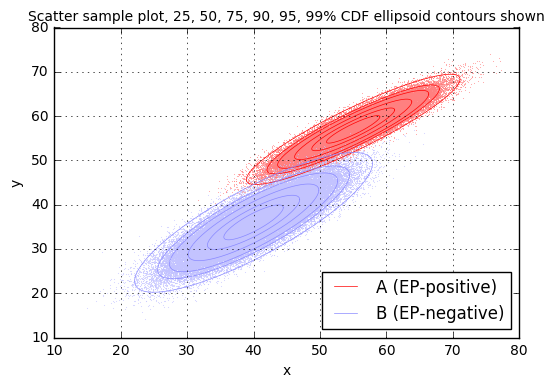
It may seem strange, but having the results of two tests (\( x \) from test \( T_1 \) and \( y \) from test \( T_2 \)) gives more useful information than the result of each test considered on its own. We’ll come back to this idea a little bit later.
The more immediate question is: given the pair of results \( (x,y) \), how would we decide whether the patient has \( EP \) or not? With just test \( T_1 \) we could merely declare an EP-positive diagnosis if \( x > x_0 \) for some threshold \( x_0 \). With two variables, some kind of inequality is involved, but how do we decide?
Bayes’ Rule
We are greatly indebted to the various European heads of state and religion during much of the 18th century (the Age of Enlightenment) for merely leaving people alone. (OK, this wasn’t universally true, but many of the monarchies turned a blind eye towards intellectualism.) This lack of interference and oppression resulted in numerous mathematical and scientific discoveries, one of which was Bayes’ Rule, named after Thomas Bayes, a British clergyman and mathematician. Bayes’ Rule was published posthumously in An Essay towards solving a Problem in the Doctrine of Chances, and later inflicted on throngs of undergraduate students of probability and statistics.
The basic idea involves conditional probabilities and reminds me of the logical converse. As a hypothetical example, suppose we know that 95% of Dairy Queen customers are from the United States and that 45% of those US residents who visit Dairy Queen like peppermint ice cream, whereas 72% of non-US residents like peppermint ice cream. We are in line to get some ice cream, and we notice that the person in front of us orders peppermint ice cream. Can we make any prediction of the probability that this person is from the US?
Bayes’ Rule relates these two conditions. Let \( A \) represent the condition that a Dairy Queen customer is a US resident, and \( B \) represent that they like peppermint ice cream. Then \( P(A\ |\ B) = \frac{P(B\ |\ A)P(A)}{P(B)} \), which is really just an algebraic rearrangement of the expression of the joint probability that \( A \) and \( B \) are both true: \( P(AB) = P(A\ |\ B)P(B) = P(B\ |\ A)P(A) \). Applied to our Dairy Queen example, we have \( P(A) = 0.95 \) (95% of Dairy Queen customers are from the US) and \( P(B\ |\ A) = 0.45 \) (45% of customers like peppermint ice cream, given that they are from the US). But what is \( P(B) \), the probability that a Dairy Queen customer likes peppermint ice cream? Well, it’s the sum of the all the constituent joint probabilities where the customer likes peppermint ice cream. For example, \( P(AB) = P(B\ |\ A)P(A) = 0.45 \times 0.95 = 0.4275 \) is the joint probability that a Dairy Queen customer is from the US and likes peppermint ice cream, and \( P(\bar{A}B) = P(B\ |\ \bar{A})P(\bar{A}) = 0.72 \times 0.05 = 0.036 \) is the joint probability that a Dairy Queen customer is not from the US and likes peppermint ice cream. Then \( P(B) = P(AB) + P(\bar{A}B) = 0.4275 + 0.036 = 0.4635 \). (46.35% of all Dairy Queen customers like peppermint ice cream.) The final application of Bayes’ Rule tells us
$$P(A\ |\ B) = \frac{P(B\ |\ A)P(A)}{P(B)} = \frac{0.45 \times 0.95}{0.4635} \approx 0.9223$$
and therefore if we see someone order peppermint ice cream at Dairy Queen, there is a whopping 92.23% chance they are not from the US.
Let’s go back to our embolary pulmonism scenario where a person takes both tests \( T_1 \) and \( T_2 \), with results \( R = (x=45, y=52) \). Can we estimate the probability that this person has EP?
N = 500000
np.random.seed(DETERMINISTIC_SEED)
xA,yA = distA.sample(N)
xB,yB = distB.sample(N)

fig=plt.figure()
ax=fig.add_subplot(1,1,1)
scatter_samples(ax,[(xA,yA,distA),
                    (xB,yB,distB)])
ax.plot(45,52,'.k');
We certainly aren’t going to be able to find the answer exactly just from looking at this chart, but it looks like an almost certain case of A being true — that is, \( R: x=45, y=52 \) implies that the patient probably has EP. Let’s figure it out as
$$P(A\ |\ R) = \frac{P(R\ |\ A)P(A)}{P(R)}.$$
Remember we said earlier that the base rate, which is the probability of any given person presenting symptoms having EP before any testing, is \( P(A) = 40\times 10^{-6} \). (This is known as the a priori probability, whenever this Bayesian stuff gets involved.) The other two probabilities \( P(R\ |\ A) \) and \( P(R) \) are technically infinitesimal, because they are part of continuous probability distributions, but we can handwave and say that \( R \) is really the condition that the results are \( 45 \le x \le 45 + dx \) and \( 52 \le y \le 52+dy \) for some infinitesimal interval widths \( dx, dy \), in which case \( P(R\ |\ A) = p_A(R)\,dx\,dy \) and \( P(R) = P(R\ |\ A)P(A) + P(R\ |\ B)P(B) = p_A(R)P(A)\,dx\,dy + p_B(R)P(B)\,dx\,dy \) where \( p_A \) and \( p_B \) are the probability density functions. Substituting this all in we get
$$P(A\ |\ R) = \frac{p_A(R)P(A)}{p_A(R)P(A)+p_B(R)P(B)}$$
The form of the bivariate normal distribution is not too complicated, just a bit unwieldy:
$$p(x,y) = \frac{1}{2\pi\sqrt{1-\rho^2}\sigma_x\sigma_y}e^{q(x,y)}$$
with
$$q(x,y) = -\frac{1}{2(1-\rho^2)}\left(\frac{(x-\mu_x)^2}{\sigma_x{}^2}-2\rho\frac{(x-\mu_x)(y-\mu_y)}{\sigma_x\sigma_y}+\frac{(y-\mu_y)^2}{\sigma_y{}^2}\right)$$
and the rest is just number crunching:
x1=45
y1=52
PA_total = 40e-6
pA = distA.pdf(x1, y1)
pB = distB.pdf(x1, y1)
print "pA(%.1f,%.1f) = %.5g" % (x1,y1,pA)
print "pB(%.1f,%.1f) = %.5g" % (x1,y1,pB)
print ("Bayes' rule result: p(A | x=%.1f, y=%.1f) = %.5g" %
       (x1,y1,pA*PA_total/(pA*PA_total+pB*(1-PA_total))))
pA(45.0,52.0) = 0.0014503 pB(45.0,52.0) = 4.9983e-07 Bayes' rule result: p(A | x=45.0, y=52.0) = 0.104
Wow, that’s counterintuitive. This result value \( R \) lies much closer to the probability “cloud” of A = EP-positive than B = EP-negative, but Bayes’ Rule tells us there’s only about a 10.4% probability that a patient with test results \( (x=45, y=52) \) has EP. And it’s because of the very low incidence of EP.
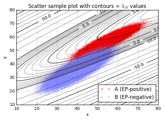
There is something we can do to make reading the graph useful, and that’s to plot a parameter I’m going to call \( \lambda(x,y) \), which is the logarithm of the ratio of probability densities:
$$\lambda(x,y) = \ln \frac{p_A(x,y)}{p_B(x,y)} = \ln p_A(x,y) - \ln p_B(x,y)$$
Actually, we’ll plot \( \lambda_{10}(x,y) = \lambda(x,y) / \ln 10 = \log_{10} \frac{p_A(x,y)}{p_B(x,y)} \).
This parameter is useful because Bayes’ rule calculates
$$\begin{aligned} P(A\ |\ x,y) &= \frac{p_A(x,y) P_A} { p_A(x,y) P_A + p_B(x,y) P_B} \cr &= \frac{p_A(x,y)/p_B(x,y) P_A} {p_A(x,y)/p_B(x,y) P_A + P_B} \cr &= \frac{e^{\lambda(x,y)} P_A} {e^{\lambda(x,y)} P_A + P_B} \cr &= \frac{1}{1 + e^{-\lambda(x,y)}P_B / P_A} \end{aligned}$$
and for any desired \( P(A\ |\ x,y) \) we can figure out the equivalent value of \( \lambda(x,y) = - \ln \left(\frac{P_A}{P_B}((1/P(A\ |\ x,y) - 1)\right). \)
This means that for a fixed value of \( \lambda \), then \( P(A\ |\ \lambda) = \frac{1}{1 + e^{-\lambda}P_B / P_A}. \)
For bivariate Gaussian distributions, the \( \lambda \) parameter is also useful because it is a quadratic function of \( x \) and \( y \), so curves of constant \( \lambda \) are conic sections (lines, ellipses, hyperbolas, or parabolas).
def jcontourp(ax,x,y,z,levels,majorfunc,color=None,fmt=None, **kwargs):
    linewidths = [1 if majorfunc(l) else 0.4 for l in levels]
    cs = ax.contour(x,y,z,levels,
                    linewidths=linewidths,
                    linestyles='-',
                    colors=color,**kwargs)
    labeled = [l for l in cs.levels if majorfunc(l)]
    ax.clabel(cs, labeled, inline=True, fmt='%s', fontsize=10)

xv = np.arange(10,80.01,0.1)
yv = np.arange(10,80.01,0.1)
x,y = np.meshgrid(xv,yv)
def lambda10(distA,distB,x,y):
    return (distA.logpdf(x, y)-distB.logpdf(x, y))/np.log(10)

fig = plt.figure()
ax = fig.add_subplot(1,1,1)
scatter_samples(ax,[(xA,yA,distA),
                    (xB,yB,distB)],
                zorder=-1)
ax.plot(x1,y1,'.k')
print "lambda10(x=%.1f,y=%.1f) = %.2f" % (x1,y1,lambda10(distA,distB,x1,y1))
levels = np.union1d(np.arange(-10,10), np.arange(-200,100,10))
def levelmajorfunc(level):
    if -10 <= level <= 10:
        return int(level) % 5 == 0
    else:
        return int(level) % 25 == 0
jcontourp(ax,x,y,lambda10(distA,distB,x,y),
          levels,
          levelmajorfunc,
          color='black')
ax.set_xlim(xv.min(), xv.max()+0.001)
ax.set_ylim(yv.min(), yv.max()+0.001)
ax.set_title('Scatter sample plot with contours = $\lambda_{10}$ values');
lambda10(x=45.0,y=52.0) = 3.46
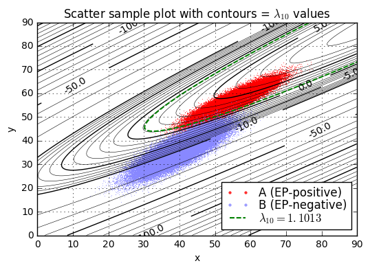
We’ll pick one particular \( \lambda_{10} \) value as a threshold \( L_{10} = L/ \ln 10 \), and if \( \lambda_{10} > L_{10} \) then we’ll declare condition \( a \) (the patient is diagnosed as EP-positive), otherwise we’ll declare condition \( b \) (the patient is diagnosed as EP-negative). The best choice of \( L_{10} \) is the one that maximizes expected value.
Remember how we did this in the case with only the one test \( T_1 \) with result \( x \): we chose threshold \( x_0 \) based on the point where \( {\partial E \over \partial x_0} = 0 \); in other words, a change in diagnosis did not change the expected value at this point. We can do the same thing here:
$$0 = {\partial E[v] \over \partial {L}} = P(A\ |\ \lambda=L)(v_{Ab}-v_{Aa}) + P(B\ |\ \lambda=L)(v_{Bb}-v_{Ba})$$
With our earlier definitions
$$\rho_v = -\frac{v_{Bb}-v_{Ba}}{v_{Ab}-v_{Aa}}, \qquad \rho_p = P_B / P_A$$
then the equation for \( L \) becomes \( 0 = P(A\ |\ \lambda=L) - \rho_v P(B\ |\ \lambda=L) = P(A\ |\ \lambda=L) - \rho_v (1-P(A\ |\ \lambda=L)) \), which simplifies to
$$P(A\ |\ \lambda=L) = \frac{\rho_v}{\rho_v+1} = \frac{1}{1+1/\rho_v} .$$
But we already defined \( \lambda \) as the group of points \( (x,y) \) that have equal probability \( P(A\ |\ \lambda) = \frac{1}{1 + e^{-\lambda}P_B / P_A} = \frac{1}{1 + \rho_p e^{-\lambda}} \) so
$$\frac{1}{1+1/\rho_v} = \frac{1}{1 + \rho_p e^{-L}}$$
which occurs when \( L = \ln \rho_v \rho_p. \)
In our EP example,
$$\begin{aligned} \rho_p &= p_B/p_A = 0.99996 / 0.00004 = 24999 \cr \rho_v &= -\frac{v_{Bb}-v_{Ba}}{v_{Ab}-v_{Aa}} = -5000 / -9.9\times 10^6 \approx 0.00050505 \cr \rho_v\rho_p &\approx 12.6258 \cr L &= \ln \rho_v\rho_p \approx 2.5357 \cr L_{10} &= \log_{10}\rho_v\rho_p \approx 1.1013 \end{aligned}$$
and we can complete the analysis empirically by looking at the fraction of pseudorandomly-generated sample points where \( \lambda_{10} < L_{10} \); this is an example of Monte Carlo analysis.
class Quadratic1D(namedtuple('Quadratic1D','a b c')):
    """
    Q(x) = a*x*x + b*x + c
    """
    __slots__ = ()
    @property
    def x0(self):
        return -self.b/(2.0*self.a)
    @property
    def q0(self):
        return self.c - self.a*self.x0**2
    def __call__(self,x):
        return self.a*x*x + self.b*x + self.c
    def solve(self, q):
        D = self.b*self.b - 4*self.a*(self.c-q)
        sqrtD = np.sqrt(D)
        return np.array([-self.b-sqrtD, -self.b+sqrtD])/(2*self.a)

class QuadraticLissajous(namedtuple('QuadraticLissajous','x0 y0 Rx Ry phi')):
    """
    A parametric curve as a function of theta:

        x = x0 + Rx * cos(theta)
        y = y0 + Ry * sin(theta+phi)
    """
    __slots__ = ()
    def __call__(self, theta):
        return (self.x0 + self.Rx * np.cos(theta),
                self.y0 + self.Ry * np.sin(theta+self.phi))

class Quadratic2D(namedtuple('Quadratic2D','a b c d e f')):
    """
    Bivariate quadratic function
    Q(x,y) = a*x*x + b*x*y + c*y*y + d*x + e*y + f
           = a*(x-x0)*(x-x0) + b*(x-x0)*(y-y0) + c*(y-y0)*(y-y0) + q0
           = s*(u*u + v*v) + q0 where s = +/-1

    https://en.wikipedia.org/wiki/Quadratic_function#Bivariate_(two_variable)_quadratic_function

    (Warning: this implementation assumes convexity,
    that is, b*b < 4*a*c, so hyperboloids/paraboloids are not handled.)
    """
    __slots__ = ()
    @property
    def discriminant(self):
        return self.b**2 - 4*self.a*self.c
    @property
    def x0(self):
        return (2*self.c*self.d - self.b*self.e)/self.discriminant
    @property
    def y0(self):
        return (2*self.a*self.e - self.b*self.d)/self.discriminant
    @property
    def q0(self):
        x0 = self.x0
        y0 = self.y0
        return self.f - self.a*x0*x0 - self.b*x0*y0 - self.c*y0*y0
    def _Kcomponents(self):
        s = 1 if self.a > 0 else -1
        r = s*self.b/2.0/np.sqrt(self.a*self.c)
        rc = np.sqrt(1-r*r)
        Kux = rc*np.sqrt(self.a*s)
        Kvx = r*np.sqrt(self.a*s)
        Kvy = np.sqrt(self.c*s)
        return Kux, Kvx, Kvy
    @property
    def Kxy2uv(self):
        Kux, Kvx, Kvy = self._Kcomponents()
        return np.array([[Kux, 0],[Kvx, Kvy]])
    @property
    def Kuv2xy(self):
        Kux, Kvx, Kvy = self._Kcomponents()
        return np.array([[1.0/Kux, 0],[-1.0*Kvx/Kux/Kvy, 1.0/Kvy]])
    @property
    def transform_xy2uv(self):
        Kxy2uv = self.Kxy2uv
        x0 = self.x0
        y0 = self.y0
        def transform(x,y):
            return np.dot(Kxy2uv, [x-x0,y-y0])
        return transform
    @property
    def transform_uv2xy(self):
        Kuv2xy = self.Kuv2xy
        x0 = self.x0
        y0 = self.y0
        def transform(u,v):
            return np.dot(Kuv2xy, [u,v]) + [[x0],[y0]]
        return transform
    def uv_radius(self, q):
        """
        Returns R such that solutions (u,v) of Q(x,y) = q
        lie within the range [-R, R],
        or None if there are no solutions.
        """
        s = 1 if self.a > 0 else -1
        D = (q-self.q0)*s
        return np.sqrt(D) if D >= 0 else None
    def _xy_radius_helper(self, q, z):
        D = (self.q0 - q) * 4 * z / self.discriminant
        if D < 0:
            return None
        else:
            return np.sqrt(D)
    def x_radius(self, q):
        """
        Returns Rx such that solutions (x,y) of Q(x,y) = q
        lie within the range [x0-Rx, x0+Rx],
        or None if there are no solutions.

        Equal to uv_radius(q)/Kux, but we can solve more directly
        """
        return self._xy_radius_helper(q, self.c)
    def y_radius(self, q):
        """
        Returns Rx such that solutions (x,y) of Q(x,y) = q
        lie within the range [x0-Rx, x0+Rx],
        or None if there are no solutions.

        Equal to uv_radius(q)/Kux, but we can solve more directly
        """
        return self._xy_radius_helper(q, self.a)
    def lissajous(self, q):
        """
        Returns a QuadraticLissajous with x0, y0, Rx, Ry, phi such that
        the solutions (x,y) of Q(x,y) = q
        can be written:

          x = x0 + Rx * cos(theta)
          y = y0 + Ry * sin(theta+phi)

        Rx and Ry and phi may each return None if no such solution exists.
        """
        D = self.discriminant
        x0 = (2*self.c*self.d - self.b*self.e)/D
        y0 = (2*self.a*self.e - self.b*self.d)/D
        q0 = self.f - self.a*x0*x0 - self.b*x0*y0 - self.c*y0*y0
        Dx = 4 * (q0-q) * self.c / D
        Rx = None if Dx < 0 else np.sqrt(Dx)
        Dy = 4 * (q0-q) * self.a / D
        Ry = None if Dy < 0 else np.sqrt(Dy)
        phi = None if D > 0 else np.arcsin(self.b / (2*np.sqrt(self.a*self.c)))
        return QuadraticLissajous(x0,y0,Rx,Ry,phi)
    def contour(self, q, npoints=360):
        """
        Returns a pair of arrays x,y such that
        Q(x,y) = q
        """
        s = 1 if self.a > 0 else -1
        R = np.sqrt((q-self.q0)*s)
        th = np.arange(npoints)*2*np.pi/npoints
        u = R*np.cos(th)
        v = R*np.sin(th)
        return self.transform_uv2xy(u,v)
    def constrain(self, x=None, y=None):
        if x is None and y is None:
            return self
        if x is None:
            # return a function in x
            return Quadratic1D(self.a,
                               self.d + y*self.b,
                               self.f + y*self.e + y*y*self.c)
        if y is None:
            # return a function in y
            return Quadratic1D(self.c,
                               self.e + x*self.b,
                               self.f + x*self.d + x*x*self.a)
        return self(x,y)
    def __call__(self, x, y):
        return (self.a*x*x
               +self.b*x*y
               +self.c*y*y
               +self.d*x
               +self.e*y
               +self.f)

def decide_limits(*args, **kwargs):
    s = kwargs.get('s', 6)
    xmin = None
    xmax = None
    for xbatch in args:
        xminb = min(xbatch)
        xmaxb = max(xbatch)
        mu = np.mean(xbatch)
        std = np.std(xbatch)
        xminb = min(mu-s*std, xminb)
        xmaxb = max(mu+s*std, xmaxb)
        if xmin is None:
            xmin = xminb
            xmax = xmaxb
        else:
            xmin = min(xmin,xminb)
            xmax = max(xmax,xmaxb)
    # Quantization
    q = kwargs.get('q')
    if q is not None:
        xmin = np.floor(xmin/q)*q
        xmax = np.ceil(xmax/q)*q
    return xmin, xmax

def separation_plot(xydistA, xydistB, Q, L, ax=None, xlim=None, ylim=None):
    L10 = L/np.log(10)
    if ax is None:
        fig = plt.figure()
        ax = fig.add_subplot(1,1,1)
    xA,yA,distA = xydistA
    xB,yB,distB = xydistB
    scatter_samples(ax,[(xA,yA,distA),
                        (xB,yB,distB)],
                    zorder=-1)

    xc,yc = Q.contour(L)
    ax.plot(xc,yc,
        color='green', linewidth=1.5, dashes=[5,2],
        label = '$\\lambda_{10} = %.4f$' % L10)
    ax.legend(loc='lower right',markerscale=10,
              labelspacing=0,fontsize=12)
    if xlim is None:
        xlim = decide_limits(xA,xB,s=6,q=10)
    if ylim is None:
        ylim = decide_limits(yA,yB,s=6,q=10)
    xv = np.arange(xlim[0],xlim[1],0.1)
    yv = np.arange(ylim[0],ylim[1],0.1)
    x,y = np.meshgrid(xv,yv)
    jcontourp(ax,x,y,lambda10(distA,distB,x,y),
              levels,
              levelmajorfunc,
              color='black')

    ax.set_xlim(xlim)
    ax.set_ylim(ylim)
    ax.set_title('Scatter sample plot with contours = $\lambda_{10}$ values')

def separation_report(xydistA, xydistB, Q, L):
    L10 = L/np.log(10)
    for x,y,dist in [xydistA, xydistB]:
        print "Separation of samples in %s by L10=%.4f" % (dist.id,L10)
        lam = Q(x,y)
        lam10 = lam/np.log(10)
        print "  Range of lambda10: %.4f to %.4f" % (np.min(lam10), np.max(lam10))
        n = np.size(lam)
        p = np.count_nonzero(lam < L) * 1.0 / n
        print "  lambda10 <  L10: %.5f" % p
        print "  lambda10 >= L10: %.5f" % (1-p)

L = np.log(5000 / 9.9e6 * 24999)
C = distA.logpdf_coefficients - distB.logpdf_coefficients
Q = Quadratic2D(*C)
separation_plot((xA,yA,distA),(xB,yB,distB), Q, L)
separation_report((xA,yA,distA),(xB,yB,distB), Q, L)
Separation of samples in A by L10=1.1013 Range of lambda10: -3.4263 to 8.1128 lambda10 < L10: 0.01760 lambda10 >= L10: 0.98240 Separation of samples in B by L10=1.1013 Range of lambda10: -36.8975 to 4.0556 lambda10 < L10: 0.99834 lambda10 >= L10: 0.00166
Or we can determine the results by numerical integration of probability density.
The math below isn’t difficult, just tedious; for each of the two Gaussian distributions for A and B, I selected a series of 5000 intervals (10001 x-axis points) from \( \mu_x-8\sigma_x \) to \( \mu_x + 8\sigma_x \), and used Simpson’s Rule to integrate the probability density \( f_x(x_i) \) at each point \( x_i \), given that
$$x \approx x_i \quad\Rightarrow\quad f_x(x) \approx f_x(x_i) = p_x(x_i) \left(F_{x_i}(y_{i2}) - F_{x_i}(y_{i1})\right)$$
where
- \( p_x(x_i) \) is the probability density that \( x=x_i \) with \( y \) unspecified
- \( F_{x_i}(y_0) \) is the 1-D cumulative distribution function, given \( x=x_i \), that \( y<y_0 \)
- \( y_{i1} \) and \( y_{i2} \) are either
- the two solutions of \( \lambda(x_i,y) = L \)
- or zero, if there are no solutions or one solution
and the sample points \( x_i \) are placed more closely together nearer to the extremes of the contour \( \lambda(x,y)=L \) to capture the suddenness of the change.
Anyway, here’s the result, which is nicely consistent with the Monte Carlo analysis:
def assert_ordered(*args, **kwargs):
    if len(args) < 2:
        return

    rthresh = kwargs.get('rthresh',1e-10)
    label = kwargs.get('label',None)
    label = '' if label is None else label+': '

    xmin = args[0]
    xmax = args[-1]
    if len(args) == 2:
        # not very interesting case
        xthresh = rthresh*(xmax+xmin)/2.0
    else:
        xthresh = rthresh*(xmax-xmin)

    xprev = xmin
    for x in args[1:]:
        assert x - xprev >= -xthresh, "%s%s > %s + %g" % (label,xprev,x,xthresh)
        xprev = x

def arccos_sat(x):
    if x <= -1:
        return np.pi
    if x >= 1:
        return 0
    return np.arccos(x)


def simpsons_rule_points(xlist, bisect=True):
    """
    Generator for Simpson's rule

    xlist:  arbitrary points in increasing order
    bisect: whether or not to add bisection points

    returns a generator of weights w (if bisect=False)
      or tuples (w,x) (if bisect = True)
    such that the integral of f(x) dx over the list of points xlist
    is approximately equal to:

    sum(w*f(x) for w,x in simpsons_rule_points(xlist))

    The values of x returned are x[i], (x[i]+x[i+1])/2, x[i+1]
    with relative weights dx/6, 4*dx/6, dx/6 for each interval
    [x[i], x[i+1]]
    """

    xiter = iter(xlist)
    xprev = xiter.next()
    w2 = 0
    x2 = None

    if bisect:
        for x2 in xiter:
            x0 = xprev
            dx = x2-x0
            x1 = x0 + dx/2.0
            xprev = x2
            w6 = dx/6.0
            w0 = w2 + w6
            yield (w0, x0)
            w1 = 4*w6
            yield (w1, x1)
            w2 = w6
        if x2 is not None:
            yield (w2, x2)
    else:
        for x1 in xiter:
            x0 = xprev
            try:
                x2 = xiter.next()
            except StopIteration:
                raise ValueError("Must have an odd number of points")
            dx = x2-x0
            xprev = x2
            w6 = dx/6.0
            w0 = w2 + w6
            yield w0
            w1 = 4*w6
            yield w1
            w2 = w6
        if x2 is not None:
            yield w2

def estimate_separation_numerical(dist, Q, L, xmin, xmax, Nintervals=5000,
                                  return_pair=False, sampling_points=None):
    """
    Numerical estimate of each row of confusion matrix
    using N integration intervals (each bisected to use Simpson's Rule)
    covering the interval [xmin,xmax].

    dist:        Gaussian2D distribution
    Q:           Quadratic2D function Q(x,y)
    L:           lambda threshold:
                   diagnose as A when Q(x,y) > L,
                   otherwise as B
    xmin:       start x-coordinate
    xmax:        end x-coordinate
    Nintervals:  number of integration intervals

    Returns p, where p is the probability of Q(x,y) > L for that
    distribution.

    If return_pair is true, returns [p,q];
    if [x1,x2] covers most of the distribution, then p+q should be close to 1.
    """
    Qliss = Q.lissajous(L)
    xqr = Qliss.Rx
    xqmu = Qliss.x0

    # Determine range of solutions:
    #    no solutions if xqr is None,
    #    otherwise Q(x,y) > L if x in Rx = [xqmu-xqr, xqmu+xqr]
    #
    # Cover the trivial cases first:

    if xqr is None:
        return (0,1) if return_pair else 0
    if (xmax < xqmu - xqr) or (xmin > xqmu + xqr):
        # All solutions are more than Nsigma from the mean
        # isigma_left  = (xqmu - xqr - dist.mu_x)/dist.sigma_x
        # isigma_right = (xqmu + xqr - dist.mu_x)/dist.sigma_x
        # print "sigma", isigma_left, isigma_right
        return (0,1) if return_pair else 0


    # We want to cover the range xmin, xmax.
    # Increase coverage near the ends of the lambda threshold,
    # xqmu +/- xqr where the behavior changes more rapidly,
    # by using points at -cos(theta) within the solution space for Q(x,y)>L


    th1 = arccos_sat(-(xmin-xqmu)/xqr)
    th2 = arccos_sat(-(xmax-xqmu)/xqr)
    # print np.array([th1,th2])*180/np.pi, xmin, xqmu-np.cos(th1)*xqr, xqmu-np.cos(th2)*xqr, xmax, (xqmu-xqr, xqmu+xqr)
    assert_ordered(xmin, xqmu-np.cos(th1)*xqr, xqmu-np.cos(th2)*xqr, xmax)

    x_arc_coverage = xqr*(np.cos(th1)-np.cos(th2))   # length along x
    x_arc_length = xqr*(th2-th1)                     # length along arc
    x_total_length = (xmax-xmin) - x_arc_coverage + x_arc_length
    x1 = xqmu-xqr*np.cos(th1)
    x2 = x1 + x_arc_length

    n = (Nintervals*2) + 1
    xlin = np.linspace(0,x_total_length, n) + xmin
    x = xlin[:]
    y = np.zeros((2,n))
    # Points along arc:
    tol = 1e-10
    i12 = (xlin >= x1 - tol) & (xlin <= x2 + tol)
    angles = th1 + (xlin[i12]-x1)/x_arc_length*(th2-th1)
    x[i12], y[0, i12] = Qliss(np.pi + angles)
    _,      y[1, i12] = Qliss(np.pi - angles)
    y.sort(axis=0)
    x[xlin >= x2] += (x_arc_coverage-x_arc_length)

    fx = dist.slicefunc('x')
    p = 0
    q = 0
    for i,wdx in enumerate(simpsons_rule_points(x, bisect=False)):
        w, mu, sigma = fx(x[i])
        y1 = y[0,i]
        y2 = y[1,i]
        cdf1 = scipy.stats.norm.cdf(y1, mu, sigma)
        cdf2 = scipy.stats.norm.cdf(y2, mu, sigma)
        deltacdf = cdf2-cdf1
        p += wdx*w*deltacdf
        q += wdx*w*(1-deltacdf)
    return (p,q) if return_pair else p

def compute_confusion_matrix(distA, distB, Q, L, Nintervals=5000, verbose=False):
    C = np.zeros((2,2))
    for i,dist in enumerate([distA,distB]):
        Nsigma = 8
        xmin = dist.mu_x - Nsigma*dist.sigma_x
        xmax = dist.mu_x + Nsigma*dist.sigma_x
        p,q = estimate_separation_numerical(dist, Q, L, xmin, xmax, Nintervals=Nintervals,
                                            return_pair=True)
        C[i,:] = [p,q]
        print "%s: p=%g, q=%g, p+q-1=%+g" % (dist.name, p,q,p+q-1)
    return C

confusion_matrix = compute_confusion_matrix(distA, distB, Q, L, verbose=True)
separation_report((xA,yA,distA),(xB,yB,distB), Q, L)
value_matrix = np.array([[0,-5000],[-1e7, -1e5]]) - 100
# Same value matrix as the original one
# (with vAb = $10 million) before but we add $100 cost for test T2

C = confusion_matrix[::-1,::-1]
# flip the confusion matrix left-right and top-bottom for B first

def gather_info(C,V,PA,**kwargs):
    info = dict(kwargs)
    C = np.array(C)
    V = np.array(V)
    info['C'] = C
    info['V'] = V
    info['J'] = C*[[1-PA],[PA]]
    return info

display(show_binary_matrix(C, 'L_{10}=%.4f' % (L/np.log(10)), [distB, distA], 'ba', 40e-6,value_matrix,
                           special_format={'v':'$%.2f'}))
info27 = gather_info(C,value_matrix,40e-6,L=L)
A (EP-positive): p=0.982467, q=0.0175334, p+q-1=-8.90805e-09 B (EP-negative): p=0.00163396, q=0.998366, p+q-1=+1.97626e-07 Separation of samples in A by L10=1.1013 Range of lambda10: -3.4263 to 8.1128 lambda10 < L10: 0.01760 lambda10 >= L10: 0.98240 Separation of samples in B by L10=1.1013 Range of lambda10: -36.8975 to 4.0556 lambda10 < L10: 0.99834 lambda10 >= L10: 0.00166
Report for threshold \(L_{10}=1.1013 \rightarrow E[v]=\)$-119.11
| b | a | |
|---|---|---|
| B (EP-negative) | 0.99837 J=0.9983263 wv=$-99.83 | 0.00163 J=0.0016339 wv=$-8.33 |
| A (EP-positive) | 0.01753 J=0.0000007 wv=$-7.01 | 0.98247 J=0.0000393 wv=$-3.93 |
There! Now we can check that we have a local maximum, by trying slightly lower and higher thresholds:
value_matrix = np.array([[0,-5000],[-1e7, -1e5]]) - 100
delta_L = 0.1*np.log(10)
for Li in [L-delta_L, L+delta_L]:
    confusion_matrix = compute_confusion_matrix(distA, distB, Q, Li, verbose=True)
    separation_report((xA,yA,distA),(xB,yB,distB), Q, Li)
    # Same value matrix before but we add $100 cost for test T2

    C = confusion_matrix[::-1,::-1]
    # flip the confusion matrix left-right and top-bottom for B first

    display(show_binary_matrix(C, 'L_{10}=%.4f' % (Li/np.log(10)),
                               [distB, distA], 'ba', 40e-6,value_matrix,
                               special_format={'v':'$%.2f'}))
A (EP-positive): p=0.984803, q=0.0151974, p+q-1=-8.85844e-09 B (EP-negative): p=0.0018415, q=0.998159, p+q-1=+2.55256e-07 Separation of samples in A by L10=1.0013 Range of lambda10: -3.4263 to 8.1128 lambda10 < L10: 0.01550 lambda10 >= L10: 0.98450 Separation of samples in B by L10=1.0013 Range of lambda10: -36.8975 to 4.0556 lambda10 < L10: 0.99819 lambda10 >= L10: 0.00181
Report for threshold \(L_{10}=1.0013 \rightarrow E[v]=\)$-119.23
| b | a | |
|---|---|---|
| B (EP-negative) | 0.99816 J=0.9981188 wv=$-99.81 | 0.00184 J=0.0018414 wv=$-9.39 |
| A (EP-positive) | 0.01520 J=0.0000006 wv=$-6.08 | 0.98480 J=0.0000394 wv=$-3.94 |
A (EP-positive): p=0.979808, q=0.0201915, p+q-1=-9.01419e-09
B (EP-negative): p=0.00144637, q=0.998554, p+q-1=+2.1961e-08
Separation of samples in A by L10=1.2013
  Range of lambda10: -3.4263 to 8.1128
  lambda10 <  L10: 0.02011
  lambda10 >= L10: 0.97989
Separation of samples in B by L10=1.2013
  Range of lambda10: -36.8975 to 4.0556
  lambda10 <  L10: 0.99850
  lambda10 >= L10: 0.00150
Report for threshold \(L_{10}=1.2013 \rightarrow E[v]=\)$-119.23
| b | a | |
|---|---|---|
| B (EP-negative) | 0.99855 J=0.9985137 wv=$-99.85 | 0.00145 J=0.0014463 wv=$-7.38 |
| A (EP-positive) | 0.02019 J=0.0000008 wv=$-8.08 | 0.97981 J=0.0000392 wv=$-3.92 |
Great! The sensitivity of threshold seems pretty flat; \( E[v] \) differs by about 12 cents if we change \( L_{10} = 1.1013 \) to \( L_{10} = 1.0013 \) or \( L_{10} = 1.2013 \). This gives us a little wiggle room in the end to shift costs between the false-negative and false-positive cases, without changing the overall expected cost very much.
Most notably, though, we’ve reduced the total cost by about \$93 by using the pair of tests \( T_1, T_2 \) compared to the test with just \( T_1 \). This is because we shift cost from the Ab (false negative for EP-positive) and Ba (false positive for EP-negative) cases to the Bb (correct for EP-negative) case — everyone has to pay \$100 more, but the chances of false positives and false negatives have been greatly reduced.
Don’t remember the statistics from the one-test case? Here they are again:
x0 = 53.1626
C = analyze_binary(dneg, dpos, x0)
value_matrix_T1 = [[0,-5000],[-1e7, -1e5]]
display(show_binary_matrix(C, x0, [dneg, dpos], 'ba', 40e-6,value_matrix_T1,
                           special_format={'v':'$%.2f'}))
info17 = gather_info(C,value_matrix_T1,40e-6,x0=x0)
Report for threshold \(x_0 = 53.1626 \rightarrow E[v]=\)$-212.52
| b | a | |
|---|---|---|
| B (EP-negative) | 0.98716 J=0.9871183 wv=$0.00 | 0.01284 J=0.0128417 wv=$-64.21 |
| A (EP-positive) | 0.36442 J=0.0000146 wv=$-145.77 | 0.63558 J=0.0000254 wv=$-2.54 |
And the equivalent cases for \( v_{Ab}= \)\$100 million:
Pa_total = 40e-6
x0 = 48.1458
C1 = analyze_binary(dneg, dpos, x0)
value_matrix_T1 = np.array([[0,-5000],[-1e8, -1e5]])
display(show_binary_matrix(C1, x0, [dneg, dpos], 'ba', Pa_total, value_matrix_T1,
                           special_format={'v':'$%.2f'}))
info18 = gather_info(C1,value_matrix_T1,Pa_total,x0=x0)

def compute_optimal_L(value_matrix,Pa_total):
    v = value_matrix
    return np.log(-(v[0,0]-v[0,1])/(v[1,0]-v[1,1])*(1-Pa_total)/Pa_total)

value_matrix_T2 = value_matrix_T1 - 100
L = compute_optimal_L(value_matrix_T2, Pa_total)
confusion_matrix = compute_confusion_matrix(distA, distB, Q, L, verbose=True)
separation_report((xA,yA,distA),(xB,yB,distB), Q, L)
# Same value matrix before but we add $100 cost for test T2

C2 = confusion_matrix[::-1,::-1]
# flip the confusion matrix left-right and top-bottom for B first

display(show_binary_matrix(C2, 'L_{10}=%.4f' % (L/np.log(10)), [distB, distA],
                           'ba', Pa_total,value_matrix_T2,
                           special_format={'v':'$%.2f'}))
separation_plot((xA,yA,distA),(xB,yB,distB), Q, L)
info28 = gather_info(C2,value_matrix_T2,Pa_total,L=L)
Report for threshold \(x_0 = 48.1458 \rightarrow E[v]=\)$-813.91
| b | a | |
|---|---|---|
| B (EP-negative) | 0.91631 J=0.9162691 wv=$0.00 | 0.08369 J=0.0836909 wv=$-418.45 |
| A (EP-positive) | 0.09796 J=0.0000039 wv=$-391.85 | 0.90204 J=0.0000361 wv=$-3.61 |
A (EP-positive): p=0.996138, q=0.00386181, p+q-1=-8.37725e-09
B (EP-negative): p=0.00491854, q=0.995081, p+q-1=+4.32711e-08
Separation of samples in A by L10=0.0973
  Range of lambda10: -3.4263 to 8.1128
  lambda10 <  L10: 0.00389
  lambda10 >= L10: 0.99611
Separation of samples in B by L10=0.0973
  Range of lambda10: -36.8975 to 4.0556
  lambda10 <  L10: 0.99514
  lambda10 >= L10: 0.00486
Report for threshold \(L_{10}=0.0973 \rightarrow E[v]=\)$-144.02
| b | a | |
|---|---|---|
| B (EP-negative) | 0.99508 J=0.9950417 wv=$-99.50 | 0.00492 J=0.0049183 wv=$-25.08 |
| A (EP-positive) | 0.00386 J=0.0000002 wv=$-15.45 | 0.99614 J=0.0000398 wv=$-3.99 |
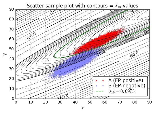
Just as in the single-test case, by changing the test threshold in the case of using both tests \( T_1+T_2 \), we’ve traded a higher confidence in using the test results for patients who are EP-positive (Ab = false negative rate decreases from about 1.75% → 0.39%) for a lower confidence in the results for patients who are EP-negative (Ba = false positive rate increases from about 0.16% → 0.49%). This and the increased cost assessment for false negatives means that the expected cost increases from \$119.11 to \$144.02 — which is still much better than the expected value from the one-test cost of \$813.91.
In numeric terms, for every 10 million patients, with 400 expected EP-positive patients, we can expect
- 393 will be correctly diagnosed as EP-positive, and 7 will be misdiagnosed as EP-negative, with \( L_{10} = 1.1013 \)
- 398 will be correctly diagnosed as EP-positive, and 2 will be misdiagnosed as EP-negative, with \( L_{10} = 0.0973 \)
(The cynical reader may conclude that, since the addition of test \( T_2 \) results in a \$670 decrease in expected cost over all potential patients, then the hospital should be charging \$770 for test \( T_2 \), not \$100.)
It’s worth noting again that we can never have perfect tests; there is always some chance of the test being incorrect. The only way to eliminate all false negatives is to increase the chances of false positives to 1. Choice of thresholds is always a compromise.
Another thing to remember is that real situations are seldom characterized perfectly by normal (Gaussian) distributions; the probability of events way out in the tails is usually higher than Gaussian because of black-swan events.
Remember: Por qué no los tres?
We’re almost done. We’ve just shown that by having everyone take both tests, \( T_1 \) and \( T_2 \), we can maximize expected value (minimize expected cost) over all patients.
But that wasn’t the original idea. Originally we were going to do this:
- Have everyone take the \$1 test \( T_1 \), which results in a measurement \( x \)
- If \( x \ge x_{H} \), diagnose as EP-positive, with no need for test \( T_2 \)
- If \( x \le x_{L} \), diagnose as EP-negative, with no need for test \( T_2 \)
- If \( x_{L} < x < x_{H} \), we will have the patient take the \$100 test \( T_2 \), which results in a measurement \( y \)
- If \( \lambda_{10}(x,y) \ge L_{10} \), diagnose as EP-positive
- If \( \lambda_{10}(x,y) < L_{10} \), diagnose as EP-negative
where \( \lambda_{10}(x,y) = \lambda(x,y) / \ln 10 = \log_{10} \frac{p_A(x,y)}{p_B(x,y)}. \)
Now we just need to calculate thresholds \( x_H \) and \( x_L \). These are going to need to have very low false positive and false negative rates, and they’re there to catch the “obvious” cases without the need to charge for (and wait for) test \( T_2 \).
We have the same kind of calculation as before. Let’s consider \( x=x_H \). It should be chosen so that with the correct threshold, there’s no change in expected value if we change the threshold by a small amount. (\( \partial E[v] / \partial x_H = 0 \)). We can do this by finding \( x_H \) such that, within a narrow range \( x_H < x < x_H+\Delta x \), the expected value is equal for both alternatives, namely whether we have them take test \( T_2 \), or diagnose them as EP-positive without taking test \( T_2 \).
Essentially we are determining thresholds \( x_H \) and \( x_L \) that, at each threshold, make the additional value of information gained from test \( T_2 \) (as measured by a change in expected value) equal to the cost of test \( T_2 \).
Remember that the total probability of \( x_H < x < x_H+\Delta x \) is \( (P_A p_A(x_H) + (1-P_A)p_B(x_H))\Delta x \), broken down into
- \( P_A p_A(x_H) \Delta x \) for EP-positive patients (A)
- \( (1-P_A) p_B(x_H) \Delta x \) for EP-negative patients (B)
Expected value \( V_1 \) for diagnosing as EP-positive (a) without taking test \( T_2 \), divided by \( \Delta x \) so we don’t have to keep writing it:
$$V_1(x_H) = P_A v_{Aa}p_A(x_H) + (1-P_A) v_{Ba} p_B(x_H)$$
where \( p_A(x), p_B(x) \) are Gaussian PDFs of the results of test \( T_1 \).
Expected value \( V_2 \) taking test \( T_2 \), which has value \( v(T_2)=-\$100 \):
$$\begin{aligned} V_2(x_0) &= v(T_2) + P_A E[v\ |\ x_0, A]p_A(x_0) + P_B E[v\ |\ x_0, B]p_B(x_0) \cr &= v(T_2) + P_A \left(v_{Aa}P_{2a}(x_0\ |\ A) + v_{Ab}P_{2b}(x_0\ |\ A)\right) p_A(x_0) \cr &+ (1-P_A)\left(v_{Ba} P_{2a}(x_0\ |\ B) + v_{Bb}P_{2b}(x_0\ | B)\right)p_B(x_0) \end{aligned}$$
where \( P_{2A}(x_0), P_{2B}(x_0) \) are the conditional probabilities of declaring the patient as EP-positive or EP-negative based on tests \( T_1, T_2 \), given that \( x=x_0 \). This happens to be the numbers we used for numerical integration in the previous section (where we were making all patients take tests \( T_1,T_2 \)).
When we have an optimal choice of threshold \( x_H \), the expected values will be equal: \( V_1(x_H) = V_2(x_H) \), because there is no advantage. If \( V_1(x_H) < V_2(x_H) \), then we haven’t chosen a good threshold, and \( x_H \) should be lower; if \( V_1(x_H) > V_2(x_H) \) then \( x_H \) should be higher. (Example: suppose that \( x_H = 55, V_1(x_H) = -400, \) and \( V_2(x_H) = -250. \) The way we’ve defined \( x_H \) is that any result of test \( T_1 \) where \( x > x_H \), the value of \( x \) is high enough that we’re better off — in other words, the expected value is supposed to be higher — just declaring diagnosis \( a \) instead of spending the extra \$100 to get a result from test \( T_2 \), given its expected value. In mathematical terms, \( V_1(x) > V_2(x) \) as long as \( x > x_H \). But we can choose \( x = x_H + \delta \) with arbitrarily small \( \delta \), and in this case we have \( V_1(x_H + \delta) > V_2(x_H+\delta) \) which contradicts \( V_1(x_H) < V_2(x_H) \). Nitpicky mathematicians: this means that the expected values \( V_1(x_H) \) and \( V_2(x_H) \) as functions of threshold \( x_H \) are continuous there. The proof should be a trivial exercise for the reader, right?)
So we just need to find the right value of \( x_H \) such that \( V_1(x_H) = V_2(x_H) \).
Presumably there is a way to determine a closed-form solution here, but I won’t even bother; we’ll just evaluate it numerically.
We’ll also cover the case where we need to find \( x_L \), where we decide just to make a diagnosis \( b \) if \( x < x_L \) based on \( T_1 \) alone, and the resulting expected value is
$$V_1(x_L) = P_A v_{Ab}p_A(x_L) + (1-P_A) v_{Bb} p_B(x_L),$$
otherwise if \( x \ge x_L \), pay the \$100 to take test \( T_2 \) with expected value \( V_2(x_L) \).
Then we just need to find \( x_L \) such that \( V_1(x_L) = V_2(x_L). \)
Let’s get an idea of what these functions look like for our example.
def compute_value_densities(which_one, distA, distB, Pa_total, value_matrix, vT2, L):
    """
    Returns a function to compute value densities V0, V1
    """
    fxA = distA.slicefunc('x')
    fxB = distB.slicefunc('x')
    vAa = value_matrix[1,1]
    vBa = value_matrix[0,1]
    vAb = value_matrix[1,0]
    vBb = value_matrix[0,0]
    if which_one == 'H':
        vA1 = vAa
        vB1 = vBa
    elif which_one == 'L':
        vA1 = vAb
        vB1 = vBb
    else:
        raise ValueError("which_one must be 'H' or 'L'")
    normcdf = scipy.stats.norm.cdf
    C = distA.logpdf_coefficients - distB.logpdf_coefficients
    Q = Quadratic2D(*C)
    Qliss = Q.lissajous(L)
    xqr = Qliss.Rx
    xqmu = Qliss.x0
    # Find the center and radius of the contour lambda(x,y)=L

    def v1v2(x_0, verbose=False):
        wA, muA, sigmaA = fxA(x_0)
        wB, muB, sigmaB = fxB(x_0)
        # wA = probability density at x = x_0 given case A
        # wB = probability density at x = x_0 given case B
        # muA, sigmaA describe the pdf p(y | A,x=x0)
        # muB, sigmaB describe the pdf p(y | B,x=x0)

        if x_0 < xqmu - xqr or x_0 > xqmu + xqr:
            # x is extreme enough that we always diagnose as "b"
            P2Aa = 0
            P2Ab = 1
            P2Ba = 0
            P2Bb = 1
        else:
            # Here we need to find the y-value thresholds
            theta = np.arccos((x_0-xqmu)/xqr)
            x1,y1 = Qliss(theta)
            x2,y2 = Qliss(-theta)
            assert np.abs(x_0-x1) < 1e-10*xqr, (x_0,x1,x2)
            assert np.abs(x_0-x2) < 1e-10*xqr, (x_0,x1,x2)
            if y1 > y2:
                y1,y2 = y2,y1
            assert np.abs(Q(x_0,y1) - L) < 1e-10
            assert np.abs(Q(x_0,y2) - L) < 1e-10
            # Diagnose as "a" if between the thresholds, otherwise "b"
            P2Aa = normcdf(y2, muA, sigmaA) - normcdf(y1, muA, sigmaA)
            P2Ab = 1-P2Aa
            P2Ba = normcdf(y2, muB, sigmaB) - normcdf(y1, muB, sigmaB)
            P2Bb = 1-P2Ba
        # expected value given the patient has results of both tests
        # over the full range of y
        vA2 = vAa*P2Aa+vAb*P2Ab    # given A, x_0
        vB2 = vBa*P2Ba+vBb*P2Bb    # given B, x_0
        # Bayes' rule for conditional probability of A and B given x_0
        PA = (Pa_total*wA)/(Pa_total*wA + (1-Pa_total)*wB)
        PB = 1-PA
        v1 =       PA*vA1 + PB*vB1
        v2 = vT2 + PA*vA2 + PB*vB2
        if verbose:
            print which_one, x_0
            print "PA|x0=",PA
            print vAa,vAb,vBa,vBb
            print P2Aa, P2Ab, P2Ba, P2Bb
            print "T1 only", vA1,vB1
            print "T1+T2  ", vA2,vB2
            print "v1=%g v2=%g v2-v1=%g" % (v1,v2,v2-v1)
        return v1,v2
    return v1v2


Pa_total = 40e-6
value_matrix_T1 = np.array([[0,-5000],[-1e7, -1e5]])
vT2 = -100
L = compute_optimal_L(value_matrix_T1 + vT2, Pa_total)
distA2 = Gaussian2D(mu_x=63,mu_y=57,sigma_x=5.3,sigma_y=4.1,rho=0.91,name='A (EP-positive)',id='A',color='red')
distB2 = Gaussian2D(mu_x=48,mu_y=36,sigma_x=5.9,sigma_y=5.2,rho=0.84,name='B (EP-negative)',id='B',color='#8888ff')

print "For L10=%.4f:" % (L/np.log(10))
for which in 'HL':
    print ""
    v1v2 = compute_value_densities(which, distA, distB, Pa_total, value_matrix_T1, vT2, L)
    for x_0 in np.arange(25,100.1,5):
        v1,v2 = v1v2(x_0)
        print "x_%s=%.1f, V1=%.4g, V2=%.4g, V2-V1=%.4g" % (which, x_0,v1,v2,v2-v1)
For L10=1.1013: x_H=25.0, V1=-5000, V2=-100, V2-V1=4900 x_H=30.0, V1=-5000, V2=-100, V2-V1=4900 x_H=35.0, V1=-5000, V2=-100.5, V2-V1=4900 x_H=40.0, V1=-5000, V2=-104.2, V2-V1=4896 x_H=45.0, V1=-5001, V2=-122.2, V2-V1=4879 x_H=50.0, V1=-5011, V2=-183.7, V2-V1=4828 x_H=55.0, V1=-5107, V2=-394.5, V2-V1=4713 x_H=60.0, V1=-5840, V2=-1354, V2-V1=4487 x_H=65.0, V1=-1.033e+04, V2=-6326, V2-V1=4008 x_H=70.0, V1=-2.878e+04, V2=-2.588e+04, V2-V1=2902 x_H=75.0, V1=-6.315e+04, V2=-6.185e+04, V2-V1=1301 x_H=80.0, V1=-8.695e+04, V2=-8.661e+04, V2-V1=339.4 x_H=85.0, V1=-9.569e+04, V2=-9.567e+04, V2-V1=26.9 x_H=90.0, V1=-9.843e+04, V2=-9.849e+04, V2-V1=-59.82 x_H=95.0, V1=-9.933e+04, V2=-9.942e+04, V2-V1=-85.24 x_H=100.0, V1=-9.967e+04, V2=-9.976e+04, V2-V1=-93.59 x_L=25.0, V1=-0.001244, V2=-100, V2-V1=-100 x_L=30.0, V1=-0.0276, V2=-100, V2-V1=-100 x_L=35.0, V1=-0.5158, V2=-100.5, V2-V1=-99.95 x_L=40.0, V1=-8.115, V2=-104.2, V2-V1=-96.09 x_L=45.0, V1=-107.5, V2=-122.2, V2-V1=-14.63 x_L=50.0, V1=-1200, V2=-183.7, V2-V1=1016 x_L=55.0, V1=-1.126e+04, V2=-394.5, V2-V1=1.087e+04 x_L=60.0, V1=-8.846e+04, V2=-1354, V2-V1=8.711e+04 x_L=65.0, V1=-5.615e+05, V2=-6326, V2-V1=5.551e+05 x_L=70.0, V1=-2.503e+06, V2=-2.588e+04, V2-V1=2.477e+06 x_L=75.0, V1=-6.121e+06, V2=-6.185e+04, V2-V1=6.059e+06 x_L=80.0, V1=-8.627e+06, V2=-8.661e+04, V2-V1=8.54e+06 x_L=85.0, V1=-9.547e+06, V2=-9.567e+04, V2-V1=9.451e+06 x_L=90.0, V1=-9.835e+06, V2=-9.849e+04, V2-V1=9.736e+06 x_L=95.0, V1=-9.93e+06, V2=-9.942e+04, V2-V1=9.83e+06 x_L=100.0, V1=-9.965e+06, V2=-9.976e+04, V2-V1=9.865e+06
import matplotlib.gridspec

def fVdistort(V):
    return -np.log(-np.array(V+ofs))

yticks0 =np.array([1,2,5])
yticks = -np.hstack([yticks0 * 10**k for k in xrange(-1,7)])

for which in 'HL':
    fig = plt.figure(figsize=(6,6))
    gs = matplotlib.gridspec.GridSpec(2,1,height_ratios=[2,1],hspace=0.1)
    ax=fig.add_subplot(gs[0])
    x = np.arange(20,100,0.2)
    fv1v2 = compute_value_densities(which, distA, distB, Pa_total, value_matrix_T1, vT2, L)

    v1v2 = np.array([fv1v2(xi) for xi in x])
    vlim = np.array([max(-1e6,v1v2.min()*1.01),
                     min(-10,v1v2.max()*0.99)])
    f = fVdistort
    ax.plot(x,f(v1v2[:,0]),label='T1 only (declare %s if $x%s$)' %
            (('"a"', '>x_H') if which == 'H' else ('"b"', '<x_L')))
    ax.plot(x,f(v1v2[:,1]),label='T1+T2')
    ax.set_yticks(f(yticks))
    ax.set_yticklabels('%.0f' % y for y in yticks)
    ax.set_ylim(f(vlim))
    ax.set_ylabel('$E[v]$',fontsize=12)
    ax.grid(True)
    ax.legend(labelspacing=0, fontsize=10,
              loc='lower left' if which=='H' else 'upper right')
    [label.set_visible(False) for label in ax.get_xticklabels()]

    ax2=fig.add_subplot(gs[1], sharex=ax)
    ax2.plot(x,v1v2[:,1]-v1v2[:,0])
    ax2.set_ylim(-500,2000)
    ax2.grid(True)
    ax2.set_ylabel('$\\Delta E[v]$')
    ax2.set_xlabel('$x_%s$' % which, fontsize=12)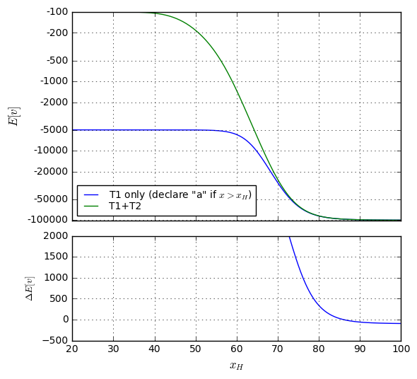
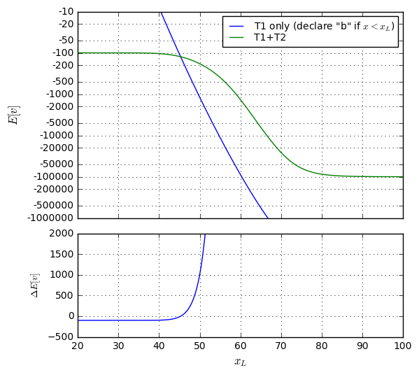
It looks like for this case (\( L_{10}=1.1013 \)), we should choose \( x_L \approx 45 \) and \( x_H \approx 86 \).
These edge cases where \( x < x_L \) or \( x > x_H \) don’t save a lot of money, at best just the \$100 \( T_2 \) test cost… so a not-quite-as-optimal but simpler case would be to always run both tests. Still, there’s a big difference between going to the doctor and paying \$1 rather than \$101… whereas once you’ve paid a \$100,000 hospital bill, what’s an extra \$100 among friends?
Between those thresholds, where test \( T_1 \) is kind of unhelpful, the benefit of running both tests is enormous: for EP-positive patients we can help minimize those pesky false negatives, saving hospitals millions in malpractice charges and helping those who would otherwise have grieving families; for EP-negative patients we can limit the false positives and save them the \$5000 and anguish of a stressful hospital stay.
Putting it all together
Now we can show our complete test protocol on one graph and one chart. Below the colored highlights show four regions:
- blue: \( b_1 \) — EP-negative diagnosis after taking test \( T_1 \) only, with \( x<x_L \)
- green: \( b_2 \) — EP-negative diagnosis after taking tests \( T_1, T_2 \), with \( x_L \le x \le x_H \) and \( \lambda_{10} < L_{10} \)
- yellow: \( a_2 \) — EP-positive diagnosis after taking tests \( T_1, T_2 \), with \( x_L \le x \le x_H \) and \( \lambda_{10} \ge L_{10} \)
- red: \( a_1 \) — EP-positive diagnosis after taking tests \( T_1 \) only, with \( x > x_H \)
import matplotlib.patches as patches
import matplotlib.path
import scipy.optimize
Path = matplotlib.path.Path

def show_complete_chart(xydistA, xydistB, Q, L, Pa_total, value_matrix_T1, vT2,
                        return_info=False):
    fig = plt.figure()
    ax = fig.add_subplot(1,1,1)
    xlim = (0,100)
    ylim = (0,100)
    separation_plot(xydistA, xydistB, Q, L, ax=ax, xlim=xlim, ylim=ylim)
    ax.set_xticks(np.arange(0,101.0,10))
    ax.set_yticks(np.arange(0,101.0,10))

    # Solve for xL and xH
    _,_,distA = xydistA
    _,_,distB = xydistB
    v1v2 = [compute_value_densities(which, distA, distB, Pa_total,
                                    value_matrix_T1, vT2, L)
            for which in 'LH']
    def fdelta(f):
        def g(x):
            y1,y2 = f(x)
            return y1-y2
        return g
    xL = scipy.optimize.brentq(fdelta(v1v2[0]), 0, 100)
    xH = scipy.optimize.brentq(fdelta(v1v2[1]), 0, 100)

    # Show the full matrix of possibilities:
    # compute 2x4 confusion matrix
    C = []
    for dist in [distB, distA]:
        distx = dist.project('x')
        pa2,pb2 = estimate_separation_numerical(dist, Q, L, xL, xH,
                                                Nintervals=2500,
                                                return_pair=True)
        row = [distx.cdf(xL), pb2, pa2, 1-distx.cdf(xH)]
        C.append(row)
    # compute 2x4 value matrix
    V = value_matrix_T1.repeat(2,axis=1)
    V[:,1:3] += vT2

    display(show_binary_matrix(confusion_matrix=C,
                       threshold='x_L=%.3f, x_H=%.3f, L_{10}=%.3f'
                                 %(xL,xH,L/np.log(10)),
                       distributions=[distB,distA],
                       outcome_ids=['b1','b2','a2','a1'],
                       ppos=Pa_total,
                       vmatrix=V,
                       special_format={'v':'$%.2f',
                                       'J':['%.8f','%.8f','%.8f','%.3g']}))

    # Highlight each of the areas
    x0,x1 = xlim
    y0,y1 = ylim
    # area b1: x < xL
    rect = patches.Rectangle((x0,y0),xL-x0,y1-y0,linewidth=0,edgecolor=None,facecolor='#8888ff',alpha=0.1)
    ax.add_patch(rect)
    # area a1: x > xH
    rect = patches.Rectangle((xH,y0),x1-xH,y1-y0,linewidth=0,edgecolor=None,facecolor='red',alpha=0.1)
    ax.add_patch(rect)
    for x in [xL,xH]:
        ax.plot([x,x],[y0,y1],color='gray')
    # area a2: lambda(x,y) > L
    xc,yc = Q.contour(L)
    ii = (xc > xL-10) & (xc < xH + 10)
    xc = xc[ii]
    yc = yc[ii]
    xc = np.maximum(xc,xL)
    xc = np.minimum(xc,xH)
    poly2a = patches.Polygon(np.vstack([xc,yc]).T, edgecolor=None, facecolor='yellow',alpha=0.5)
    ax.add_patch(poly2a)

    # area b2: lambda(x,y) < L
    xy = []
    op = []
    i = 0
    for x,y in zip(xc,yc):
        i += 1
        xy.append((x,y))
        op.append(Path.MOVETO if i == 1 else Path.LINETO)
    xy.append((0,0))
    op.append(Path.CLOSEPOLY)
    xy += [(xL,y0),(xL,y1),(xH,y1),(xH,y0),(0,0)]
    op += [Path.MOVETO, Path.LINETO, Path.LINETO, Path.LINETO, Path.CLOSEPOLY]
    patch2b = patches.PathPatch(Path(xy,op), edgecolor=None, facecolor='#00ff00',alpha=0.1)
    ax.add_patch(patch2b)

    # add labels
    style = {'fontsize': 28, 'ha':'center'}

    ax.text((x0+xL)/2,y0*0.3+y1*0.7,'$b_1$', **style)
    ax.text(xc.mean(), yc.mean(), '$a_2$', **style)
    a = 0.3 if yc.mean() > (x0+x1)/2 else 0.7
    yb2 = a*y1 + (1-a)*y0
    ax.text(xc.mean(), yb2, '$b_2$',**style)
    xa1 = (xH + x1) / 2
    ya1 = max(30, min(90, Q.constrain(x=xa1).x0))
    ax.text(xa1,ya1,'$a_1$',**style)

    if return_info:
        C = np.array(C)
        J = C * [[1-Pa_total],[Pa_total]]
        return dict(C=C,J=J,V=V,xL=xL,xH=xH,L=L)

value_matrix_T1 = np.array([[0,-5000],[-1e7, -1e5]])
value_matrix_T2 = value_matrix_T1 - 100
L = compute_optimal_L(value_matrix_T2, Pa_total)
info37 = show_complete_chart((xA,yA,distA),(xB,yB,distB), Q, L, Pa_total,
                            value_matrix_T1, vT2, return_info=True)
Report for threshold \(x_L=45.287, x_H=85.992, L_{10}=1.101 \rightarrow E[v]=\)$-46.88
| b1 | b2 | a2 | a1 | |
|---|---|---|---|---|
| B (EP-negative) | 0.81491 J=0.81487784 wv=$0.00 | 0.18377 J=0.18376595 wv=$-18.38 | 0.00132 J=0.00131622 wv=$-6.71 | 0.00000 J=3.22e-15 wv=$-0.00 |
| A (EP-positive) | 0.03343 J=0.00000134 wv=$-13.37 | 0.01148 J=0.00000046 wv=$-4.59 | 0.95509 J=0.00003820 wv=$-3.82 | 0.00000 J=9.98e-14 wv=$-0.00 |
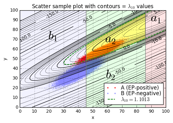
We can provide the same information but with the false negative cost (Ab = wrongly diagnosed EP-negative) at \$100 million:
value_matrix_T1 = np.array([[0,-5000],[-1e8, -1e5]])
value_matrix_T2 = value_matrix_T1 - 100
L = compute_optimal_L(value_matrix_T2, Pa_total)
info38 = show_complete_chart((xA,yA,distA),(xB,yB,distB), Q, L, Pa_total,
                            value_matrix_T1, vT2, return_info=True)
Report for threshold \(x_L=40.749, x_H=85.108, L_{10}=0.097 \rightarrow E[v]=\)$-99.60
| b1 | b2 | a2 | a1 | |
|---|---|---|---|---|
| B (EP-negative) | 0.55051 J=0.55048511 wv=$0.00 | 0.44489 J=0.44486873 wv=$-44.49 | 0.00461 J=0.00460618 wv=$-23.49 | 0.00000 J=1.04e-14 wv=$-0.00 |
| A (EP-positive) | 0.00358 J=0.00000014 wv=$-14.34 | 0.00333 J=0.00000013 wv=$-13.30 | 0.99309 J=0.00003972 wv=$-3.98 | 0.00000 J=2.68e-13 wv=$-0.00 |
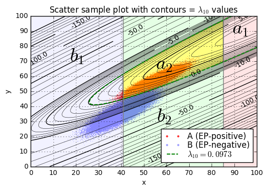
Do we need test \( T_1 \)?
If adding test \( T_2 \) is so much better than test \( T_1 \) alone, why do we need test \( T_1 \) at all? What if we just gave everyone test \( T_2 \)?
y = np.arange(0,100,0.1)
distA_T2 = distA.project('y')
distB_T2 = distB.project('y')
show_binary_pdf(distA_T2, distB_T2, y, xlabel = '$T_2$ test result $y$')

for false_negative_cost in [10e6, 100e6]:
    value_matrix_T2 = np.array([[0,-5000],[-false_negative_cost, -1e5]]) - 100
    threshold_info = find_threshold(distB_T2, distA_T2, Pa_total, value_matrix_T2)
    y0 = [yval for yval,_ in threshold_info if yval > 20 and yval < 80][0]

    C = analyze_binary(distB_T2, distA_T2, y0)
    print "False negative cost = $%.0fM" % (false_negative_cost/1e6)
    display(show_binary_matrix(C, 'y_0=%.2f' % y0, [distB_T2, distA_T2], 'ba', Pa_total, value_matrix_T2,
                       special_format={'v':'$%.2f'}))
    info = gather_info(C,value_matrix_T2,Pa_total,y0=y0)
    if false_negative_cost == 10e6:
        info47 = info
    else:
        info48 = info
False negative cost = $10M
Report for threshold \(y_0=50.14 \rightarrow E[v]=\)$-139.03
| b | a | |
|---|---|---|
| B (EP-negative) | 0.99673 J=0.9966899 wv=$-99.67 | 0.00327 J=0.0032701 wv=$-16.68 |
| A (EP-positive) | 0.04717 J=0.0000019 wv=$-18.87 | 0.95283 J=0.0000381 wv=$-3.82 |
False negative cost = $100M
Report for threshold \(y_0=47.73 \rightarrow E[v]=\)$-211.68
| b | a | |
|---|---|---|
| B (EP-negative) | 0.98795 J=0.9879069 wv=$-98.79 | 0.01205 J=0.0120531 wv=$-61.47 |
| A (EP-positive) | 0.01187 J=0.0000005 wv=$-47.47 | 0.98813 J=0.0000395 wv=$-3.96 |

Hmm. That seems better than the \( T_1 \) test… but the confusion matrix doesn’t seem as good as using both tests.
d prime \( (d’) \): Are two tests are always better than one?
Why would determining a diagnosis based on both tests \( T_1 \) and \( T_2 \) be better than from either test alone?
Let’s graph the PDFs of three different measurements:
- \( x \) (the result of test \( T_1 \))
- \( y \) (the result of test \( T_2 \))
- \( u = -0.88x + 1.88y \) (a linear combination of the two measurements)
We’ll also calculate a metric for each of the three measurements,
$$d’ = \frac{\mu_A - \mu_B}{\sqrt{\frac{1}{2}(\sigma_A{}^2 + \sigma_B{}^2)}}$$
which is a measure of the “distinguishability” between two populations which each have normal distributions. Essentially it is a unitless “separation coefficient” that measures the distances between the means as a multiple of the “average” standard deviation. It is also invariant under scaling and translation — if we figure out the value of \( d’ \) for some measurement \( x \), then any derived measurement \( u = ax + c \) has the same value for \( d’ \) as long as \( a \ne 0 \).
(We haven’t talked about derived measurements like \( u \), but for a 2-D Gaussian distribution, if \( u=ax+by+c \) then:
$$\begin{aligned} \mu_u &= E[u] = aE[x]+bE[y] = a\mu_x + b\mu_y + c\cr \sigma_u{}^2 &= E[(u-\mu_u)^2] \cr &= E[a^2(x-\mu_x)^2 + 2ab(x-\mu_x)(y-\mu_y) + b^2(y-\mu_y)^2] \cr &= a^2E[(x-\mu_x)^2] + 2abE[(x-\mu_x)(y-\mu_y)] + b^2E[(y-\mu_y)^2] \cr &= a^2 \sigma_x{}^2 + 2ab\rho\sigma_x\sigma_y + b^2\sigma_y{}^2 \end{aligned}$$
or, alternatively using matrix notation, \( \sigma_u{}^2 = \mathrm{v}^T \mathrm{S} \mathrm{v} \) where \( \mathrm{v} = \begin{bmatrix}a& b\end{bmatrix}^T \) is the vector of weighting coefficients, and \( \mathrm{S} = \operatorname{cov}(x,y) = \begin{bmatrix}\sigma_x{}^2 & \rho\sigma_x\sigma_y \cr \rho\sigma_x\sigma_y & \sigma_y{}^2\end{bmatrix} \). Yep, there’s the covariance matrix again.)
def calc_dprime(distA,distB,projection):
    """ calculates dprime for two distributions,
    given a projection P = [cx,cy]
    that defines u = cx*x + cy*y
    """
    distAp = distA.project(projection)
    distBp = distB.project(projection)
    return (distAp.mu - distBp.mu)/np.sqrt(
              (distAp.sigma**2 + distBp.sigma**2)/2.0
             )

def show_dprime(distA, distB, a,b):
    print "u=%.6fx%+.6fy" % (a,b)
    x = np.arange(0,100,0.1)
    fig = plt.figure()
    ax = fig.add_subplot(1,1,1)
    for projname, projection, linestyle in [
        ('x','x',':'),
        ('y','y','--'),
        ('u',[a,b],'-')]:
        distAp = distA.project(projection)
        distBp = distB.project(projection)
        dprime = calc_dprime(distA, distB, projection)
        print "dprime(%s)=%.4f" % (projname,dprime)
        for dist in [distAp,distBp]:
            ax.plot(x,dist.pdf(x),
                    color=dist.color,
                    linestyle=linestyle,
                    label='$%s$: %s, $\\mu=$%.1f, $\\sigma=$%.2f' %
                        (projname, dist.id, dist.mu, dist.sigma))
    ax.set_ylabel('probability density')
    ax.set_xlabel('measurement $(x,y,u)$')
    ax.set_ylim(0,0.15)
    ax.legend(labelspacing=0, fontsize=10,loc='upper left');

show_dprime(distA, distB, -0.88,1.88)
u=-0.880000x+1.880000y dprime(x)=2.6747 dprime(y)=4.4849 dprime(u)=5.1055
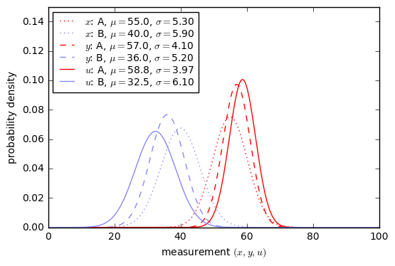
We can get a better separation between alternatives, as measured by \( d’ \), through this linear combination of \( x \) and \( y \) than by either one alone. What’s going on, and where did the equation \( u=-0.88x + 1.88y \) come from?
Can we do better than that? How about \( u=-0.98x + 1.98y \)? or \( u=-0.78x + 1.78y \)?
show_dprime(distA, distB, -0.98,1.98)
u=-0.980000x+1.980000y
dprime(x)=2.6747
dprime(y)=4.4849
dprime(u)=5.0997

show_dprime(distA, distB, -0.78,1.78)
u=-0.780000x+1.780000y
dprime(x)=2.6747
dprime(y)=4.4849
dprime(u)=5.0988
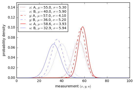
Hmm. These aren’t quite as good; the value for \( d’ \) is lower. How do we know how to maximize \( d’ \)?
Begin grungy algebra
There doesn’t look like a simple intuitive way to find the best projection. At first I thought of modeling this as \( v = x \cos\theta + y \sin\theta \) for some angle \( \theta \). But this didn’t produce any easy answer. I muddled my way to an answer by looking for patterns that helped to cancel out some of the grunginess.
One way to maximize \( d’ \) is to write it as a function of \( \theta \) with \( v=ax+by, a = a_1\cos \theta+a_2\sin\theta, b = b_1\cos\theta+b_2\sin\theta \) for some convenient \( a_1, a_2, b_1, b_2 \) to make the math nice. We’re going to figure out \( d’ \) as a function of \( a,b \) in general first:
$$\begin{aligned} d’ &= \frac{\mu_{vA} - \mu_{vB}}{\sqrt{\frac{1}{2}(\sigma_{vA}{}^2 + \sigma_{vB}{}^2)}} \cr &= \frac{a(\mu_{xA}-\mu_{xB})+b(\mu_{yA} - \mu_{yB})}{\sqrt{\frac{1}{2}(a^2(\sigma_{xA}^2 + \sigma_{xB}^2) + 2ab(\rho_A\sigma_{xA}\sigma_{yA} + \rho_B\sigma_{xB}\sigma_{yB}) + b^2(\sigma_{yA}^2+\sigma_{yB}^2))}} \cr &= \frac{a(\mu_{xA}-\mu_{xB})+b(\mu_{yA} - \mu_{yB})}{\sqrt{\frac{1}{2}f(a,b)}} \cr \end{aligned}$$
with \( f(a,b) = a^2(\sigma_{xA}^2 + \sigma_{xB}^2) + 2ab(\rho_A\sigma_{xA}\sigma_{yA} + \rho_B\sigma_{xB}\sigma_{yB}) + b^2(\sigma_{yA}^2+\sigma_{yB}^2). \)
Yuck.
Anyway, if we can make the denominator constant as a function of \( \theta \), then the numerator is easy to maximize.
If we define
$$\begin{aligned} K_x &= \sqrt{\sigma_{xA}^2 + \sigma_{xB}^2} \cr K_y &= \sqrt{\sigma_{yA}^2 + \sigma_{yB}^2} \cr R &= \frac{\rho_A\sigma_{xA}\sigma_{yA} + \rho_B\sigma_{xB}\sigma_{yB}}{K_xK_y} \end{aligned}$$
then \( f(a,b) = a^2K_x{}^2 + 2abRK_xK_y + b^2K_y{}^2 \) which is easier to write than having to carry around all those \( \mu \) and \( \sigma \) terms.
If we let \( a = \frac{1}{\sqrt{2}K_x}(c \cos \theta + s \sin\theta) \) and \( b = \frac{1}{\sqrt{2}K_y}(c \cos \theta - s\sin\theta) \) then
$$\begin{aligned} f(a,b) &= \frac{1}{2}(c^2 \cos^2\theta + s^2\sin^2\theta + 2cs\cos\theta\sin\theta) \cr &+ \frac{1}{2}(c^2 \cos^2\theta + s^2\sin^2\theta - 2cs\cos\theta\sin\theta) \cr &+R(c^2 \cos^2\theta - s^2\sin^2\theta) \cr &= (1+R)c^2 \cos^2\theta + (1-R)s^2\sin^2\theta \end{aligned}$$
which is independent of \( \theta \) if \( (1+R)c^2 = (1-R)s^2 \). If we let \( c = \cos \phi \) and \( s=\sin \phi \) then some nice things all fall out:
- \( f(a,b) \) is constant if \( \tan^2\phi = \frac{1+R}{1-R} \), in other words \( \phi = \tan^{-1} \sqrt{\frac{1+R}{1-R}} \)
- \( c = \cos\phi = \sqrt{\frac{1-R}{2}} \) (hint: use the identities \( \sec^2 \theta = \tan^2 \theta + 1 \) and \( \cos \theta = 1/\sec \theta \))
- \( s = \sin\phi = \sqrt{\frac{1+R}{2}} \)
- \( f(a,b) = (1-R^2)/2 \)
- \( a = \frac{1}{\sqrt{2}K_x}\cos (\theta - \phi) = \frac{1}{\sqrt{2}K_x}(\cos \phi \cos \theta + \sin\phi \sin\theta)= \frac{1}{2K_x}(\sqrt{1-R} \cos \theta + \sqrt{1+R} \sin\theta) \)
- \( b = \frac{1}{\sqrt{2}K_y}\cos (\theta + \phi) = \frac{1}{\sqrt{2}K_y}(\cos \phi \cos \theta - \sin\phi \sin\theta)= \frac{1}{2K_y}(\sqrt{1-R} \cos \theta - \sqrt{1+R} \sin\theta) \)
and when all is said and done we get
$$\begin{aligned} d’ &= \frac{a(\mu_{xA}-\mu_{xB})+b(\mu_{yA} - \mu_{yB})}{\sqrt{\frac{1}{2}f(a,b)}} \cr &= \frac{a(\mu_{xA}-\mu_{xB})+b(\mu_{yA} - \mu_{yB})}{\frac{1}{2}\sqrt{1-R^2}} \cr &= K_c \cos\theta + K_s \sin\theta \end{aligned}$$
if
$$\begin{aligned} \delta_x &= \frac{\mu_{xA}-\mu_{xB}}{K_x} = \frac{\mu_{xA}-\mu_{xB}}{\sqrt{\sigma_{xA}^2 + \sigma_{xB}^2}} \cr \delta_y &= \frac{\mu_{yA} - \mu_{yB}}{K_y} = \frac{\mu_{yA} - \mu_{yB}}{\sqrt{\sigma_{yA}^2 + \sigma_{yB}^2}} \cr K_c &= \sqrt{\frac{1-R}{1-R^2}} \left(\delta_x + \delta_y \right) \cr &= \frac{1}{\sqrt{1+R}} \left(\delta_x + \delta_y \right) \cr K_s &= \sqrt{\frac{1+R}{1-R^2}} \left(\delta_x - \delta_y \right) \cr &= \frac{1}{\sqrt{1-R}} \left(\delta_x - \delta_y \right) \cr \end{aligned}$$
Then \( d’ \) has a maximum value of \( D = \sqrt{K_c{}^2 + K_s{}^2} \) at \( \theta = \tan^{-1}\dfrac{K_s}{K_c} \), where \( \cos \theta = \dfrac{K_c}{\sqrt{K_s^2 + K_c^2}} \) and \( \sin \theta = \dfrac{K_s}{\sqrt{K_s^2 + K_c^2}}. \)
Plugging into \( a \) and \( b \) we get
$$\begin{aligned} a &= \frac{1}{2K_x}(\sqrt{1-R} \cos \theta + \sqrt{1+R} \sin\theta)\cr &= \frac{1}{2K_x}\left(\frac{(1-R)(\delta_x+\delta_y)}{\sqrt{1-R^2}}+\frac{(1+R)(\delta_x-\delta_y)}{\sqrt{1-R^2}}\right)\cdot\frac{1}{\sqrt{K_s^2 + K_c^2}} \cr &= \frac{\delta_x - R\delta_y}{K_xD\sqrt{1-R^2}}\cr b &= \frac{1}{2K_y}(\sqrt{1-R} \cos \theta - \sqrt{1+R} \sin\theta)\cr &= \frac{1}{2K_y}\left(\frac{(1-R)(\delta_x+\delta_y)}{\sqrt{1-R^2}}-\frac{(1+R)(\delta_x-\delta_y)}{\sqrt{1-R^2}}\right)\cdot\frac{1}{\sqrt{K_s^2 + K_c^2}} \cr &= \frac{-R\delta_x + \delta_y}{K_yD\sqrt{1-R^2}} \end{aligned}$$
We can also solve \( D \) in terms of \( \delta_x, \delta_y, \) and \( R \) to get
$$\begin{aligned} D &= \frac{1}{\sqrt{1-R^2}}\sqrt{(1-R)(\delta_x+\delta_y)^2 + (1+R)(\delta_x-\delta_y)^2} \cr &= \sqrt{\frac{2\delta_x^2 -4R\delta_x\delta_y + 2\delta_y^2}{1-R^2}} \cr a &= \frac{\delta_x - R\delta_y}{K_x\sqrt{2\delta_x^2 -4R\delta_x\delta_y + 2\delta_y^2}} \cr b &= \frac{-R\delta_x + \delta_y}{K_y\sqrt{2\delta_x^2 -4R\delta_x\delta_y + 2\delta_y^2}} \end{aligned}$$
Let’s try it!
Kx = np.hypot(distA.sigma_x,distB.sigma_x)
Ky = np.hypot(distA.sigma_y,distB.sigma_y)
R = (distA.rho*distA.sigma_x*distA.sigma_y + distB.rho*distB.sigma_x*distB.sigma_y)/Kx/Ky
Kx, Ky, R
(7.9309520235593407, 6.6219332524573211, 0.86723211589363869)
dmux = (distA.mu_x - distB.mu_x)/Kx
dmuy = (distA.mu_y - distB.mu_y)/Ky
Kc = (dmux + dmuy)/np.sqrt(1+R)
Ks = (dmux - dmuy)/np.sqrt(1-R)
Kc,Ks
(3.7048851247525367, -3.5127584699841927)
theta = np.arctan(Ks/Kc)
a = 1.0/2/Kx*(np.sqrt(1-R)*np.cos(theta) + np.sqrt(1+R)*np.sin(theta) )
b = 1.0/2/Ky*(np.sqrt(1-R)*np.cos(theta) - np.sqrt(1+R)*np.sin(theta) )
dprime = np.hypot(Kc,Ks)
dprime2 = Kc*np.cos(theta) + Ks*np.sin(theta)
assert abs(dprime - dprime2) < 1e-7
delta_x = (distA.mu_x - distB.mu_x)/np.hypot(distA.sigma_x,distB.sigma_x)
delta_y = (distA.mu_y - distB.mu_y)/np.hypot(distA.sigma_y,distB.sigma_y)
dd = np.sqrt(2*delta_x**2 - 4*R*delta_x*delta_y + 2*delta_y**2)
dprime3 = dd/np.sqrt(1-R*R)
assert abs(dprime - dprime3) < 1e-7
a2 = (delta_x - R*delta_y)/Kx/dd
b2 = (-R*delta_x + delta_y)/Ky/dd
assert abs(a-a2) < 1e-7
assert abs(b-b2) < 1e-7
print "theta=%.6f a=%.6f b=%.6f d'=%.6f" % (theta, a, b, dprime)
# scale a,b such that their sum is 1.0
print "   also a=%.6f b=%.6f is a solution with a+b=1" % (a/(a+b), b/(a+b))
theta=-0.758785 a=-0.042603 b=0.090955 d'=5.105453
   also a=-0.881106 b=1.881106 is a solution with a+b=1
And out pops \( u\approx -0.88x + 1.88y \).
End grungy algebra
What if we use \( u=-0.8811x + 1.8811y \) as a way to combine the results of tests \( T_1 \) and \( T_2 \)? Here is a superposition of lines with constant \( u \):
# Lines of constant u
fig = plt.figure()
ax = fig.add_subplot(1,1,1)
separation_plot((xA,yA,distA),(xB,yB,distB), Q, L, ax=ax)
xmax = ax.get_xlim()[1]
ymax = ax.get_ylim()[1]
ua = a/(a+b)
ub = b/(a+b)
for u in np.arange(ua*xmax,ub*ymax+0.01,10):
    x1 = min(xmax,(u-ub*ymax)/ua)
    x0 = max(0,u/ua)
    x = np.array([x0,x1])
    ax.plot(x,(u-ua*x)/ub,color='orange')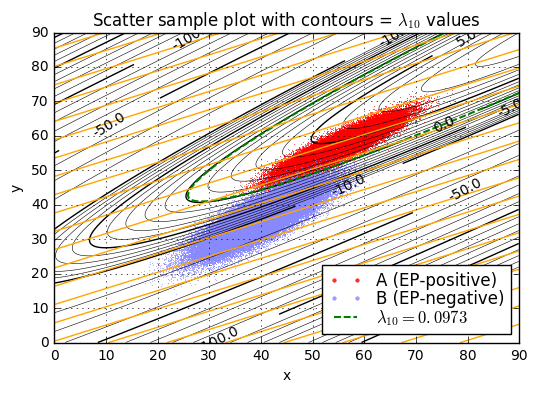
To summarize:
$$\begin{aligned} R &= \frac{\rho_A\sigma_{xA}\sigma_{yA} + \rho_B\sigma_{xB}\sigma_{yB}}{\sqrt{(\sigma_{xA}^2 + \sigma_{xB}^2)(\sigma_{yA}^2 + \sigma_{yB}^2)}} \cr \delta_x &= \frac{\mu_{xA}-\mu_{xB}}{\sqrt{\sigma_{xA}^2 + \sigma_{xB}^2}} \cr \delta_y &= \frac{\mu_{yA} - \mu_{yB}}{\sqrt{\sigma_{yA}^2 + \sigma_{yB}^2}} \cr \max d’ = D &= \sqrt{\frac{2\delta_x^2 -4R\delta_x\delta_y + 2\delta_y^2}{1-R^2}} \cr a&= \frac{\delta_x - R\delta_y}{K_x\sqrt{2\delta_x^2 -4R\delta_x\delta_y + 2\delta_y^2}}\cr b&= \frac{-R\delta_x + \delta_y}{K_y\sqrt{2\delta_x^2 -4R\delta_x\delta_y + 2\delta_y^2}}\cr \end{aligned}$$
and we can calculate a new derived measurement \( u=ax+by \) which has separation coefficient \( d’ \) between its distributions under the conditions \( A \) and \( B \).
u = np.arange(0,100,0.1)
projAB = [-0.8811, 1.8811]
distA_T1T2lin = distA.project(projAB)
distB_T1T2lin = distB.project(projAB)
show_binary_pdf(distA_T1T2lin, distB_T1T2lin, y,
                xlabel = '$u = %.4fx + %.4fy$' % tuple(projAB))

for false_negative_cost in [10e6, 100e6]:
    value_matrix_T2 = np.array([[0,-5000],[-false_negative_cost, -1e5]]) - 100
    threshold_info = find_threshold(distB_T1T2lin, distA_T1T2lin, Pa_total, value_matrix_T2)
    u0 = [uval for uval,_ in threshold_info if uval > 20 and uval < 80][0]

    C = analyze_binary(distB_T1T2lin, distA_T1T2lin, u0)
    print "False negative cost = $%.0fM" % (false_negative_cost/1e6)
    display(show_binary_matrix(C, 'u_0=ax+by=%.2f' % u0,
                               [distB_T1T2lin, distA_T1T2lin],
                               'ba', Pa_total, value_matrix_T2,
                       special_format={'v':'$%.2f'}))
    info = gather_info(C,value_matrix_T2,Pa_total,u0=u0)
    if false_negative_cost == 10e6:
        info57 = info
    else:
        info58 = info
False negative cost = $10M
Report for threshold \(u_0=ax+by=50.42 \rightarrow E[v]=\)$-119.26
| b | a | |
|---|---|---|
| B (EP-negative) | 0.99835 J=0.9983106 wv=$-99.83 | 0.00165 J=0.0016494 wv=$-8.41 |
| A (EP-positive) | 0.01771 J=0.0000007 wv=$-7.08 | 0.98229 J=0.0000393 wv=$-3.93 |
False negative cost = $100M
Report for threshold \(u_0=ax+by=48.22 \rightarrow E[v]=\)$-144.54
| b | a | |
|---|---|---|
| B (EP-negative) | 0.99504 J=0.9949981 wv=$-99.50 | 0.00496 J=0.0049619 wv=$-25.31 |
| A (EP-positive) | 0.00394 J=0.0000002 wv=$-15.74 | 0.99606 J=0.0000398 wv=$-3.99 |

One final subtlety
Before we wrap up the math, there’s one more thing that is worth a brief mention.
When we use both tests with the quadratic function \( \lambda(x,y) \), there’s a kind of funny region we haven’t talked about. Look on the graph below, at point \( P = (x=40, y=70) \):
fig = plt.figure()
ax = fig.add_subplot(1,1,1)
separation_plot((xA,yA,distA),(xB,yB,distB), Q, L, ax=ax)
P=Coordinate2D(40,70)
ax.plot(P.x,P.y,'.',color='orange')
Ptext = Coordinate2D(P.x-10,P.y)
ax.text(Ptext.x,Ptext.y,'$P$',fontsize=20,
        ha='right',va='center')
ax.annotate('',xy=P,xytext=Ptext,
            arrowprops=dict(facecolor='black',
                            width=1,
                            headwidth=5,
                            headlength=8,
                            shrink=0.05));
This point is outside the contour \( \lambda_{10} > L_{10} \), so that tells us we should give a diagnosis of EP-negative. But this point is closer to the probability “cloud” of EP-positive. Why?
for dist in [distA, distB]:
    print("Probability density at P of %s = %.3g"
          % (dist.name, dist.pdf(P.x,P.y)))
    print(dist)
Probability density at P of A (EP-positive) = 6.28e-46 Gaussian(mu_x=55, mu_y=57, sigma_x=5.3, sigma_y=4.1, rho=0.91, name='A (EP-positive)', id='A', color='red') Probability density at P of B (EP-negative) = 2.8e-34 Gaussian(mu_x=40, mu_y=36, sigma_x=5.9, sigma_y=5.2, rho=0.84, name='B (EP-negative)', id='B', color='#8888ff')
The probability density is smaller at P for the EP-positive case, even though this point is closer to the corresponding probability distribution. This is because the distribution is narrower; \( \sigma_x \) and \( \sigma_y \) are both smaller for the EP-positive case.
As a thought experiment, imagine the following distributions A and B, where B is very wide (\( \sigma=5 \)) compared to A (\( \sigma = 0.5 \)):
dist_wide = Gaussian1D(20,5,'B (wide)',id='B',color='green')
dist_narrow = Gaussian1D(25,0.5,'A (narrow)',id='A',color='red')
x = np.arange(0,40,0.1)
show_binary_pdf(dist_wide, dist_narrow, x)
plt.xlabel('x');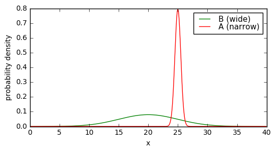
In this case, if we take some sample measurement \( x \), a classification of \( A \) makes sense only if the measured value \( x \) is near \( A \)’s mean value \( \mu=25 \), say from 24 to 26. Outside that range, a classification of \( B \) makes sense, not because the measurement is closer to the mean of \( B \), but because the expected probability of \( B \) given \( x \) is greater. This holds true even for values within a few standard deviations from the mean, like \( x=28 = \mu_B + 1.6\sigma_B \), because the distribution of \( A \) is so narrow.
We’ve been proposing tests where there is a single threshold — for example diagnose as \( a \) if \( x > x_0 \), otherwise diagnose as \( b \) — but there are fairly simple cases where two thresholds are required. In fact, this is true in general when the standard deviations are unequal; if you get far enough away from the means, the probability of the wider distribution is greater.
You might think, well, that’s kind of strange, if I’m using the same piece of equipment to measure all the sample data, why would the standard deviations be different? A digital multimeter measuring voltage, for example, has some inherent uncertainty. But sometimes the measurement variation is due to differences in the populations themselves. For example, consider the wingspans of two populations of birds, where \( A \) consists of birds that are pigeons and \( B \) consists of birds that are not pigeons. The \( B \) population will have a wider range of measurements simply because this population is more heterogeneous.
Please note, by the way, that the Python functions I wrote to analyze the bivariate Gaussian situation make the assumption that the standard deviations are unequal and the log-likelihood ratio \( \lambda(x,y) \) is either concave upwards or concave downwards — in other words, the \( A \) distribution has lower values of both \( \sigma_x \) and \( \sigma_y \) than the \( B \) distribution, or it has higher values of both \( \sigma_x \) and \( \sigma_y \). In these cases, the contours of constant \( \lambda \) are ellipses. In general, they may be some other conic section (lines, parabolas, hyperbolas) but I didn’t feel like trying to achieve correctness in all cases, for the purposes of this article.
So which test is best?
Let’s summarize the tests we came up with. We have 10 different tests, namely each of the following with false-negative costs of \$10 million and \$100 million:
- test \( T_1 \) only
- tests \( T_1 \) and \( T_2 \) – quadratic function of \( x,y \)
- test \( T_1 \) first, then \( T_2 \) if needed
- test \( T_2 \) only
- tests \( T_1 \) and \( T_2 \) – linear function of \( x,y \)
import pandas as pd

def present_info(info):
    C = info['C']
    J = info['J']
    V = info['V']
    if 'x0' in info:
        threshold = '\\( x_0 = %.2f \\)' % info['x0']
        t = 1
        Bb1 = J[0,0]
        Bb2 = 0
    elif 'xL' in info:
        threshold = ('\\( x_L = %.2f, x_H=%.2f, L_{10}=%.4f \\)'
                   % (info['xL'],info['xH'],info['L']/np.log(10)))
        t = 3
        Bb1 = J[0,0]
        Bb2 = J[0,1]
    elif 'L' in info:
        threshold = '\\( L_{10}=%.4f \\)' % (info['L']/np.log(10))
        t = 2
        Bb1 = 0
        Bb2 = J[0,0]
    elif 'y0' in info:
        threshold = '\\( y_0 = %.2f \\)' % info['y0']
        t = 4
        Bb1 = 0
        Bb2 = J[0,0]
    elif 'u0' in info:
        threshold = '\\( u_0 = ax+by = %.2f \\)' % info['u0']
        t = 4
        Bb1 = 0
        Bb2 = J[0,0]
    nc = J.shape[1]
    return {'Exp. cost':'$%.2f' % (-J*V).sum(),
            'Threshold': threshold,
            'N(Ab)': int(np.round(10e6*J[1,:nc//2].sum())),
            'N(Ba)': int(np.round(10e6*J[0,nc//2:].sum())),
            'N(Aa)': int(np.round(10e6*J[1,nc//2:].sum())),
            'P(b|A)': '%.2f%%' % (C[1,:nc//2].sum() * 100),
            'P(Bb,$0)': '%.2f%%' % (Bb1*100),
            'P(Bb,$100)': '%.2f%%' % (Bb2*100),
        }

tests = ['\\(T_1\\)',
         '\\(T_1 + T_2\\)',
         '\\(T_1 \\rightarrow T_2 \\)',
         '\\(T_2\\)',
         '\\(T_1 + T_2\\) (linear)']
print "Exp. cost = expected cost above test T1 ($1)"
print "N(Aa) = expected number of correctly-diagnosed EP-positives per 10M patients"
print "N(Ab) = expected number of false negatives per 10M patients"
print "N(Ba) = expected number of false positives per 10M patients"
print("P(Bb,$0)   = percentage of patients correctly diagnosed EP-negative,\n"+
      "             no additional cost after test T1")
print("P(Bb,$100) = percentage of patients correctly diagnosed EP-negative,\n"+
      "             test T2 required")
print "P(b|A) = conditional probability of a false negative for EP-positive patients"
print "T1 -> T2:   test T1 followed by test T2 if needed"
df = pd.DataFrame([present_info(info)
             for info in [info17,info27,info37,info47,info57,
                          info18,info28,info38,info48,info58]],
             index=['\\$%dM, %s' % (cost,test)
                    for cost in [10,100]
                    for test in tests])
colwidths = [12,10,7,7,10,10,10,10,24]
colwidthstyles = [{'selector':'thead th.blank' if i==0
                               else 'th.col_heading.col%d' % (i-1),
                  'props':[('width','%d%%'%w)]}
             for i,w in enumerate(colwidths)]
df.style.set_table_styles([{'selector':' ','props':
                            {'width':'100%',
                             'table-layout':'fixed',
                             }.items()},
                           {'selector':'thead th',
                            'props':[('font-size','90%')]},
                           {'selector':
                            'td span.MathJax_CHTML,td span.MathJax,th span.MathJax_CHTML,th span.MathJax',
                            'props':[('white-space','normal')]},
                           {'selector':'td.data.col7',
                            'props':[('font-size','90%')]}]
                          + colwidthstyles)
Exp. cost = expected cost above test T1 ($1)
N(Aa) = expected number of correctly-diagnosed EP-positives per 10M patients
N(Ab) = expected number of false negatives per 10M patients
N(Ba) = expected number of false positives per 10M patients
P(Bb,$0) = percentage of patients correctly diagnosed EP-negative,
no additional cost after test T1
P(Bb,$100) = percentage of patients correctly diagnosed EP-negative,
test T2 required
P(b|A) = conditional probability of a false negative for EP-positive patients
T1 -> T2: test T1 followed by test T2 if needed
| Exp. cost | N(Aa) | N(Ab) | N(Ba) | P(Bb,$0) | P(Bb,$100) | P(b|A) | Threshold | |
|---|---|---|---|---|---|---|---|---|
| \$10M, \(T_1\) | $212.52 | 254 | 146 | 128417 | 98.71% | 0.00% | 36.44% | \( x_0 = 53.16 \) |
| \$10M, \(T_1 + T_2\) | $119.11 | 393 | 7 | 16339 | 0.00% | 99.83% | 1.75% | \( L_{10}=1.1013 \) |
| \$10M, \(T_1 \rightarrow T_2 \) | $46.88 | 382 | 18 | 13162 | 81.49% | 18.38% | 4.49% | \( x_L = 45.29, x_H=85.99, L_{10}=1.1013 \) |
| \$10M, \(T_2\) | $139.03 | 381 | 19 | 32701 | 0.00% | 99.67% | 4.72% | \( y_0 = 50.14 \) |
| \$10M, \(T_1 + T_2\) (linear) | $119.26 | 393 | 7 | 16494 | 0.00% | 99.83% | 1.77% | \( u_0 = ax+by = 50.42 \) |
| \$100M, \(T_1\) | $813.91 | 361 | 39 | 836909 | 91.63% | 0.00% | 9.80% | \( x_0 = 48.15 \) |
| \$100M, \(T_1 + T_2\) | $144.02 | 398 | 2 | 49183 | 0.00% | 99.50% | 0.39% | \( L_{10}=0.0973 \) |
| \$100M, \(T_1 \rightarrow T_2 \) | $99.60 | 397 | 3 | 46062 | 55.05% | 44.49% | 0.69% | \( x_L = 40.75, x_H=85.11, L_{10}=0.0973 \) |
| \$100M, \(T_2\) | $211.68 | 395 | 5 | 120531 | 0.00% | 98.79% | 1.19% | \( y_0 = 47.73 \) |
| \$100M, \(T_1 + T_2\) (linear) | $144.54 | 398 | 2 | 49619 | 0.00% | 99.50% | 0.39% | \( u_0 = ax+by = 48.22 \) |
There! We can keep expected cost down by taking the \( T_1 \rightarrow T_2 \) approach (test 2 only if \( x_L \le x \le x_H \)).
With \$10M cost of a false negative, we can expect over 81% of patients will be diagnosed correctly as EP-negative with just the \$1 cost of the eyeball photo test, and only 18 patients out of ten million (4.5% of EP-positive patients) will experience a false negative.
With \$100M cost of a false negative, we can expect over 55% of patients will be diagnosed correctly as EP-negative with just the \$1 cost of the eyeball photo test, and only 3 patients out of ten million (0.7% of EP-positive patients) will experience a false negative.
And although test \( T_2 \) alone is better than test \( T_1 \) alone, both in keeping expected costs down, and in reducing the incidence of both false positives and false negatives, it’s pretty clear that relying on both tests is the most attractive option.
There is not too much difference between the combination of tests \( T_1+T_2 \) using \( \lambda_{10}(x,y) > L_{10} \) as a quadratic function of \( x \) and \( y \) based on the logarithm of the probability density functions, and a linear function \( u = ax+by > u_0 \) for optimal choices of \( a,b \). The quadratic function has a slightly lower expected cost.
What the @%&^ does this have to do with embedded systems?
We’ve been talking a lot about the mathematics of binary classification based on a two-test set of measurements with measurement \( x \) from test \( T_1 \) and measurement \( y \) from test \( T_2 \), where the probability distributions over \( (x,y) \) are a bivariate normal (Gaussian) distribution with slightly different values of mean \( (\mu_x, \mu_y) \) and covariance matrix \( \begin{bmatrix}\sigma_x{}^2 & \rho\sigma_x\sigma_y \cr \rho\sigma_x\sigma_y & \sigma_y{}^2\end{bmatrix} \) for two cases \( A \) and \( B \).
As an embedded system designer, why do you need to worry about this?
Well, you probably don’t need the math directly. It is worth knowing about different ways to use the results of the tests.
The more important aspect is knowing that a binary outcome based on continuous measurements throws away information. If you measure a sensor voltage and sound an alarm if the sensor voltage \( V > V_0 \) but don’t sound the alarm if \( V \le V_0 \) then this doesn’t distinguish the case of \( V \) being close to the threshold \( V_0 \) from the case where \( V \) is far away from the threshold. We saw this with idiot lights. Consider letting users see the original value \( V \) as well, not just the result of comparing it with the threshold. Or have two thresholds, one indicating a warning and the second indicating an alarm. This gives the user more information.
Be aware of the tradeoffs in choosing a threshold — and that someone needs to choose a threshold. If you lower the false positive rate, the false negative rate will increase, and vice versa.
Finally, although we’ve emphasized the importance of minimizing the chance of a false negative (in our fictional embolary pulmonism example, missing an EP-positive diagnosis may cause the patient to die), there are other costs to false positives besides inflicting unnecessary costs on users/patients. One that occurs in the medical industry is “alarm fatigue”, which is basically a loss of confidence in equipment/tests that cause frequent false positives. It is the medical device equivalent to the Aesop’s fable about the boy who cried wolf. One 2011 article stated it this way:
In one case, at UMass Memorial Medical Center in Worcester, nurses failed to respond to an alarm that sounded for about 75 minutes, signaling that a patient’s heart monitor battery needed to be replaced. The battery died, so when the patient’s heart failed, no crisis alarm sounded.
In another instance at Massachusetts General Hospital last year, an elderly man suffered a fatal heart attack while the crisis alarm on his cardiac monitor was turned off and staff did not respond to numerous lower-level alarms warning of a low heart rate. Nurses told state investigators they had become desensitized to the alarms.
“If you have that many alarms going off all the time, they lose their ability to work as an alarm,” Schyve said.
One solution may be to abandon the ever-present beep and use sounds that have been designed to reduce alarm fatigue.
The real takeaway here is that the human-factors aspect of a design (how an alarm is presented) is often as important or even more important than the math and engineering behind the design (how an alarm is detected). This is especially important in safety-critical situations such as medicine, aviation, nuclear engineering, or industrial machinery.
References
- The accuracy of yes/no classification, University of Pennsylvania
- Sensitivity and Bias - an introduction to Signal Detection Theory, University of Birmingham
- Signal Detection Theory, New York University
- D-prime (signal detection) analysis, University of California at Los Angeles
- Calculation of signal detection theory measures, Stanislaw and Todorov, Behavior Research Methods, Instruments, & Computers, March 1999
Wrapup
We’ve talked in great detail today about binary outcome tests, where one or more continuous measurements are used to detect the presence of some condition \( A \), whether it’s a disease, or an equipment failure, or the presence of an intruder.
- False positives are when the detector erroneously signals that the condition is present. (consequences: annoyance, lost time, unnecessary costs and use of resources)
- False negatives are when the detector erroneously does not signal that the condition is present. (consequences: undetected serious conditions that may get worse)
- Choice of a threshold can trade off false positive and false negative rates
- Understanding the base rate (probability that the condition occurs) is important to avoid the base rate fallacy
- If the probability distribution of the measurement is a normal (Gaussian) distribution, then an optimal threshold can be chosen to maximize expected value, by using the logarithm of the probability density function (PDF), given:
- the first- and second-order statistics (mean and standard deviation for single-variable distributions) of both populations with and without condition \( A \)
- knowledge of the base rate
- estimated costs of all four outcomes (true positive detection, false positive, false negative, true negative)
- A binary outcome test can be examined in terms of a confusion matrix that shows probabilities of all four outcomes
- We can find the optimal threshold by knowing that if a measurement occurs at the optimal threshold, both positive and negative diagnoses have the same expected value, based the conditional probability of occurrence given the measured value
- Bayes’ Rule can be used to compute the conditional probability of \( A \) given the measured value, from its “converse”, the conditional probability of the measured value with and without condition \( A \)
- Idiot lights, where the detected binary outcome is presented instead of the original measurement, hide information from the user, and should be used with caution
- The distinguishability or separation coefficient \( d’ \) can be used to characterize how far apart two probability distributions are, essentially measuring the difference of the means, divided by an effective standard deviation
- If two tests are possible, with an inexpensive test \( T_1 \) offering a mediocre value of \( d’ \), and a more expensive test \( T_2 \) offering a higher value of \( d’ \), then the two tests can be combined to help reduce overall expected costs. We explored one situation (the fictional “embolary pulmonism” or EP) where the probability distribution was a known bivariate normal distribution. Five methods were used, in order of increasing effectiveness:
- Test \( T_1 \) only, producing a measurement \( x \), detecting condition \( A \) if \( x>x_0 \) (highest expected cost)
- Test \( T_2 \) only, producing a measurement \( y \), detecting condition \( A \) if \( y>y_0 \)
- Test \( T_1 \) and \( T_2 \), combined by a linear combination \( u = ax+by \), detecting condition \( A \) if \( u>u_0 \), with \( a \) and \( b \) chosen to maximize \( d’ \)
- Test \( T_1 \) and \( T_2 \), combined by a quadratic function \( \lambda(x,y) = a(x-\mu_x)^2 + b(x-\mu_x)(y-\mu_y) + c(y-\mu_y)^2 \) based on the log of the ratio of PDFs, detecting condition \( A \) if \( \lambda(x,y) > L \) (in our example, this has a slightly lower cost than the linear combination)
- Test \( T_1 \) used to detect three cases based on thresholds \( x_L \) and \( x_H \) (lowest expected cost):
- Diagnose absense of condition \( A \) if \( x < x_L \), no further test necessary
- Diagnose presence of condition \( A \) if \( x > x_H \), no further test necessary
- If \( x_L \le x \le x_H \), perform test \( T_2 \) and diagnose based on the measurements from both tests (we explored using the quadratic function in this article)
- An excessive false positive rate can cause “alarm fatigue” in which true positives may be missed because of a tendency to ignore detected conditions
Whew! OK, that’s all for now.
© 2019 Jason M. Sachs, all rights reserved.


- Comments
- Write a Comment Select to add a comment
To post reply to a comment, click on the 'reply' button attached to each comment. To post a new comment (not a reply to a comment) check out the 'Write a Comment' tab at the top of the comments.
Please login (on the right) if you already have an account on this platform.
Otherwise, please use this form to register (free) an join one of the largest online community for Electrical/Embedded/DSP/FPGA/ML engineers: