A Second Look at Slew Rate Limiters

I recently had to pick a slew rate for a current waveform, and I got this feeling of déjà vu… hadn’t I gone through this effort already? So I looked, and lo and behold, way back in 2014 I wrote an article titled Slew Rate Limiters: Nonlinear and Proud of It! where I explored the effects of two types of slew rate limiters, one feedforward and one feedback, given a particular slew rate \( R \).

Here was one figure I published at the time:

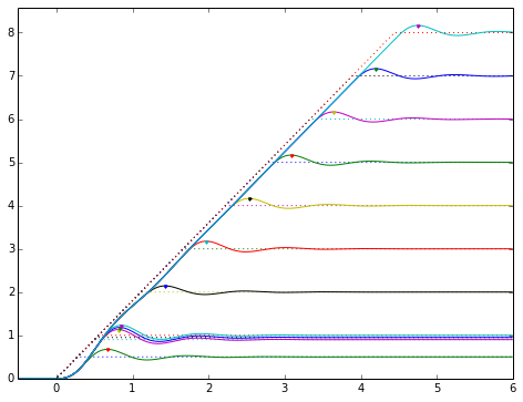
This shows a second-order system response for various step sizes that have been fed through a feedforward slew rate limiter. You’ll note the slew rate is constant — again, the idea was to explore the implications of using some given slew rate.

Great! That’s a big part of why I write these articles, so when I figure out how to deal with some little aspect of circuit design or signal processing, I can file it away on EmbeddedRelated, and then when Future Me scratches his head and looks around online… hey, look, there’s another article Jason wrote on the subject already… I’d better thank this guy, as he’s saved me a lot of unnecessary effort.

But now in 2022, I need to choose a slew rate for a fixed step size. So today I’ll show you a quick look at that and come up with a fairly easy rule to follow.

Problem Statement for Today

To be more precise:

Suppose you have a signal input \( x(t) \) that you control, and it needs to go from some initial value \( x_0 \) to some final value \( x_1 = x_0 + \Delta x \) with some slew rate \( R \).

This signal goes into a second-order system \( H(s) = \dfrac{1}{\tau^2s^2 + 2\zeta\tau s + 1} = \dfrac{{\omega_n}^2}{s^2 + 2\zeta\omega_n s + {\omega_n}^2} \), and out comes \( y(t) \).

Suppose also that this system has a little bit of overshoot (\( \zeta < 1/\sqrt{2} \approx 0.7071 \)), and I’d like to choose slew rate \( R \) to reduce the overshoot a bit, while not adding too much delay for the output reaching its final value.

We’re going to use the normalized second-order system \( H(\bar{s}) = \dfrac{1}{\bar{s}^2 + 2\zeta\bar{s} + 1} \) with \( \bar{s} = \tau s = s/\omega_n \), and drop the overbar, so we don’t have to mess around with any of that omega or tau business.

I’m not going to bother with an analytical solution today; that’s possible, but sometimes I just like working with numerical analysis to find an empirical solution, and feel like leaving the Grungy Algebra for another day.

scipy/numpy/matplotlib to the Rescue

I had to reinstall Anaconda Python recently to deal with a library issue, so I’ve finally taken the leap to use Python 3 on my home computer. (I went through this pain in the last two years at work. It’s not too bad — like ripping off a bandaid — as long as you don’t have a lot of legacy programs to deal with, and even then, you can always run Python 2 if you want)

My advice if you’re going through this:

• Start with miniconda (earlier version installers at https://repo.anaconda.com/miniconda/) which is a minimal package install, and then you can install whatever you want afterwards.
  • If this is for commercial use: version 4.7.12.1 is the last version with a bsd3 installer. (Newer installers have a more restrictive license. The Python installation itself is open-source, but not the installer.)
  • If it’s for home use, just use the latest version.
  • I had to manually update my .bash_profile on OS X to add ~/opt/miniconda3/condabin to my path
  • You can run conda init bash (or other shell name if you’re using another shell) to get your shell to default to the base environment.

• Install mamba: Anaconda Python is great, but when you want to install new packages, conda goes through this compatibility-checking step which has become extremely slow, taking minutes or hours in some cases. (Actually, I don’t know about hours, I just gave up after 5-10 minutes.) The mamba project re-implemented the compatibility-checking step in C++ for speed.

  conda install mamba -c conda-forge
  

• Learn to use conda environments! They’re basically compartmentalized installations so you can control the particular set of Python packages used in each case. I have three main environments:

  • the base environment, which remains minimalist (I don’t generally install new packages here)
  • one for Python 2
  • one for Python 3

  If I want to try a new Python package speculatively without messing up my existing environments, I create a new environment first, so I can test it out there before adding it into my main environments.

• To make your installation compatible with Jupyter (IPython Notebook), you’ll want to install nb_conda_kernels in your base environment, and ipykernel in any other environment that you want to use from Jupyter. Then you can run ipython notebook or jupyter notebook in your base environment and choose the kernel from the list.

  • Main environment: mamba install nb_conda_kernels -c conda-forge
  • Client environments: mamba install ipykernel and then for some reason I had to install mamba install decorator=4.4.0 to get around an error.

• Common packages worth installing for numerical analysis:

  • numpy
  • scipy
  • matplotlib
  • numba
  • pandas

Okay, enough of that little digression. Let’s run some code!

import matplotlib.pyplot as plt
import numpy as np
%matplotlib inline

from scipy.signal import lsim, lti

def zeta_from_ov(ov):
    '''Given an amount of overshoot,
    returns the value of zeta that causes that
    overshoot in a second-order system with no zeros.'''
    lnov = np.log(ov)
    return -lnov/np.sqrt(np.pi**2 + lnov**2)

def ratelimitedstep(slewrate, initval=0.0, finalval=1.0):
    T_end = (finalval - initval) * 1.0 / slewrate
    A = (finalval-initval) / 2.0 / T_end
    B = (finalval+initval) / 2.0 
    def f(t):
        return A*(np.abs(t) - np.abs(t-T_end)) + B
    return f

def interpolate_max(y, t, N=5):
    """
    Find a discrete maximum of a waveform 
    and interpolate with a quadratic fit for more accuracy 
    for smooth functions.
    
    y:  array of values
    t:  array of time values at which y occurs
    N:  neighborhood size
    """
    i = np.argmax(y)
    ii = slice(i-N,i+N+1)
    
    # Select t,y in neighborhood of maximum
    tn = t[ii]
    yn = y[ii]
    
    # Linear scaling of t to the interval -1,1
    # for numerical conditioning
    k0 = (tn[0] + tn[-1])/2.0
    k1 = (tn[-1] - tn[0])/2.0
    u = (tn-k0)/k1

    basis = np.vstack([np.ones_like(u), u, u*u])
    coeffs = np.linalg.lstsq(basis.T, yn.T, rcond=-1)[0]
    u0 = -coeffs[1]/(2*coeffs[2])   # vertex of quadratic = -b/2a
    y0 = coeffs[0] + u0*coeffs[1] + u0*u0*coeffs[2]
    x0 = u0*k1 + k0
    return x0, y0

def _test_interpolate():
    t0 = np.arange(0.35,0.94,0.005)
    t=t0**1.5
    def f(t):
        return np.sin(t*2) * np.exp(-2*t)
    y = f(t)
    plt.figure(figsize=(8,6))
    plt.plot(t,y,'.')
    t1 = np.arange(0.12,0.85,0.001)
    plt.plot(t1,f(t1),linewidth=0.8)
    x0,y0 = interpolate_max(y,t)
    plt.plot(x0,y0,'x')
    plt.grid(True)
    plt.ylim(0.315,0.325)
    plt.xlim(0.35,0.45)
    print("expected max x0,y0=(%.5f,%.7f)" % (x0,y0))
    eps = 1e-3
    print("f(x) in small neighborhood about x0:(%.7f,%.7f,%.7f)" % (f(x0-eps),f(x0),f(x0+eps)))
    
#_test_interpolate()

def test_case(ov):
    zeta = zeta_from_ov(ov)
    H = lti([1],[1, 2*zeta, 1])
    
    dt = 0.002
    t = np.arange(0,22,dt)
    fig = plt.figure(figsize=(9,7))
    ax = fig.add_subplot(1,1,1)
    k0 = 10
    Z = 2*np.pi
    for k in range(25):
        r = None if k == 0 else k0/k/2/np.pi
        if r is None:
            t2, y = H.step(T=t)
            u = t>0
        else:
            f = ratelimitedstep(r)
            u = f(t)
            t2, y, _ = lsim(H,u,t)
        kwargs = {} if k > 0 and k != k0 else {'color':'black'}
        lw = 1.5 if k == k0 else 0.8
        hl = ax.plot(t2/Z,y,linewidth=lw,**kwargs)
        c = hl[0].get_color()
        ax.plot(t/Z,u,'--',linewidth=lw,color=c)
        t0, y0 = interpolate_max(y,t2)
        if k == 0:
            t0noslew = t0
        if k == k0:
            t_a, y_a = t0, y0
        ax.plot(t0/Z,y0,'x' if k == k0 else '.', color=c)
    ax.set_xlim(min(t/Z),max(t/Z))
    ax.grid(True)
    ax.set_xlabel('Time ($t/2\\pi\\tau$)')
    ax.set_ylabel('Response')
    ax.set_title('Step response of a slew-rate-limited unit step with %.1f%% overshoot ($\\zeta=%.4f$)\n'
                  % (ov*100,zeta) +
                 'Time to reach final input in units $2\\pi\\tau/10$; %.1f%% overshoot with peak delayed %.2f$\\tau$'
                  % ((y_a-1)*100,t_a - t0noslew))
    
for ov in [0.05, 0.1, 0.2, 0.4, 0.6]:
    test_case(ov)

My conclusion is that a good choice for slew rate \( R = \Delta x/T \) where \( T = 2\pi\alpha\tau \) is the time to slew from initial to final value, and \( \alpha \) is some empirical choice, is with \( \alpha = 1 \). This is the thick black dotted line (input) and thick black curve (output) in the above graphs.

For higher values of zeta (smaller overshoot: say, \( \zeta > 0.5 \), which corresponds to overshoot below about 16.3%):

• For \( \alpha = 1 \), overshoot gets reduced by a factor of about 3 - 3.5, and the peak gets delayed by about \( 5\tau \)
• There’s a clear tradeoff between a faster response and higher overshoot, vs. a slower response with less overshoot. Values of \( \alpha \) in the 0.7 to 1.0 range are about right.

For lower values of zeta (larger overshoot: \( \zeta < 0.5 \)):

• The choice \( \alpha = 1 \) is more optimal; lower slew rates (values of \( \alpha > 1 \)) either have diminishing returns to decrease the overshoot, or can actually increase the overshoot.
• Overshoot gets limited to the 5.7% - 7.8% range, and the peak gets delayed by about \( 4.7\tau - 5.0\tau \)

Just as an example, suppose I wanted to ramp voltage from 3.0V to 5.0V, with a second-order system having \( \tau = 100 \mu s \) and \( \zeta = 0.4559 \) (20% overshoot step response; this is shown in one of the graphs above)

With a step in voltage command, the output would reach a maximum of 5.4V (20% overshoot of a 2V step) at about \( t=\pi\tau = 314\mu s \).

If I choose \( R=\Delta V/2\pi\alpha\tau \) with \( \alpha=1 \), I get \( R=3.183 \) V/ms, and I would expect an overshoot of about 5.4% → 5.11 V, delayed about 500 μs from the no-slew-rate-limit case, putting the peak about 814 μs.

Let’s simulate it, along with a faster slew rate, say \( R= \) 5 V/ms:

zeta = 0.4559
tau = 100e-6
H = lti([1],[tau*tau, 2*zeta*tau, 1])
        
dt = 10e-6
t = np.arange(0,0.0015,dt)
V0 = 3
V1 = 5

fig = plt.figure(figsize=(9,7))
ax = fig.add_subplot(1,1,1)

for R in [None, 5e3, 3.183e3]:
    if R is None:
        u = (V1-V0)*(t>0)+V0
    else:
        f = ratelimitedstep(R,initval=3.0,finalval=5.0)
        u = f(t)
    # subtract out initial value and add it back in,
    # because I don't feel like figuring out initial state conditions
    t1, y1, _ = lsim(H,u-V0,t)
    y1 += V0

    hl = ax.plot(t1*1e3,y1,label='output (no slew rate limit)' if R is None
                            else 'output (R=%.3fV/ms)' % (R/1000))
    c = hl[0].get_color()
    ax.plot(t*1e3,u,linestyle='--',color=c)
    tmax, ymax = interpolate_max(y1,t1)
    ax.plot(tmax*1e3,ymax,'.',color=c)
    ax.text(tmax*1e3,ymax+0.015,'%.3f V' % ymax, ha='center')
ax.legend()
ax.grid(True)
ax.set_xlim(min(t)*1e3,max(t)*1e3)
ax.set_xlabel('Time (ms)')

Text(0.5, 0, 'Time (ms)')

OK, great! Just about what we predicted!

I have analyzed only the feedforward slew rate limiter here, not the feedback slew rate limiter I showed in my earlier article.

Wrapup

If you’re adding a slew rate limiter to help reduce overshoot in a second-order system with time constant \( \tau \) and damping factor \( \zeta \) (this assumes that you aren’t tuning it more conservatively to increase \( \zeta \) and reduce the overshoot, for other reasons), then a good choice of slew rate limit is \( R = \dfrac{\Delta x}{2\pi\alpha\tau} \) with \( \alpha\approx 1 \) for a step input of \( \Delta x \).

Got an interesting signal processing issue that you’d like to learn more about? Let me know!

© 2022 Jason M. Sachs, all rights reserved.