


Slew Rate Limiters: Nonlinear and Proud of It!
I first learned about slew rate limits when I was in college. Usually the subject comes up when talking about the nonideal behavior of op-amps. In order for the op-amp output to swing up and down quickly, it has to charge up an internal capacitor with a transistor circuit that’s limited in its current capability. So the slew rate limit \( \frac{dV}{dt} = \frac{I_{\rm max}}{C} \). And as long as the amplitude and frequency aren’t too high, you won’t notice it. But try to output a square wave? BAH HA HA HA HA! Those nice fast edges that you’d like to see will slow down.
import numpy as np
import matplotlib.pyplot as plt

def ratelimit(x,t,rlim):
    def helper():
        y = x[0]
        tprev = t[0]
        for (xi,ti) in zip(x,t):
            dy = xi - y
            dt = ti - tprev
            y += np.clip(dy,-rlim*dt,rlim*dt)
            tprev = ti
            yield y
    return np.array(list(helper()))

t = np.arange(0,2,0.001)
sqwave = np.mod(t,1) > 0.5
maxslew = 10.0
out = ratelimit(sqwave, t, maxslew)
plt.plot(t,sqwave,':',t,out)
plt.ylim(-0.1,1.1)
plt.legend(['in','out'],'best')
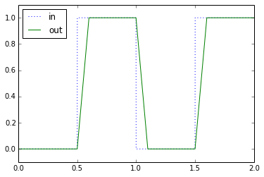
We don’t like slew-rate limits in hardware because they represent distortion. Nonlinearity! Look what happens if we put double the amplitude of a square wave with a slew-rate limit:
plt.plot(t,sqwave,':',t,out,t,sqwave*2,':',t,ratelimit(sqwave*2,t,maxslew))
plt.ylim(-0.2,2.2)
plt.legend(['in 1','out 1','in 2','out 2'],'best')
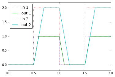
Double the amplitude, and you double the time needed to slew from one value to the other. That’s a nonlinear effect: if slew-rate limiting were linear, doubling the input would double the output, and hence double the rate of change of the output. No dice, Q.E.D.
Slew-rate limiting isn’t only something that shows up in op-amps. It can occur in any dynamic system — electrical, mechanical, pneumatic, hydraulic, chemical, etc. — where the rate of change of the system state is constrained. It happens a lot with actuators. And there’s not much else to say about actuators. You get what you get.
And sometimes we even add our own slew rate limits to a system.
Adding a Slew Rate Limit On Purpose
Now why would we want to add a slew rate on purpose? We don’t like this nonlinearity when we’re stuck with it; why would we want to add it ourselves? If we want a square wave, let’s get a square wave, not this lame trapezoidal thing.
Except for one thing: sometimes we have systems where there are costs or constraints that relate to how fast something changes. And that something may not have a nice built-in slew rate limit. Blah blah blah, boring generalization. Mea culpa. Okay, here’s a specific example:
Suppose you are closing a door. It takes you what, maybe a second from start to finish? You probably don’t even think about all the trajectory planning your brain does automatically when you go to close the door.
Now close it twice as fast. Half a second. Okay, no big deal, it just feels faster than normal. How about five times faster: 0.2 seconds. Could you do it? Maybe. But look what happens:
- The door closing will be louder.
- The door closing will vibrate more, and maybe damage something in the door hinge or the door frame.
- You will have to use 5× the force you normally would.
- When the door closes, you might hurt your hand from the impact.
- You will have less precise control of closing the door.
- You could lose your balance.
- You might pull or strain a muscle.
You might not be able to close the door that fast; the force you can exert on the door may be inherently slew-rate limited by your muscle strength. That’s inherent slew-rate limiting in an actuator. But if that’s not the case, then one of the preceding effects might occur, and these represent costs or consequences that occur before reaching the inherent slew rate limit. The only thing preventing these effects is your ability to control how you close a door.
This happens all the time with muscle movement. You almost never try to command a step trajectory in the way your body moves; instead, it’s a smooth. continuous movement.
In electrical systems the analogy is to charge up a capacitor, where faster rates of voltage change require higher currents. In mechanical systems the analogy is to move something with inertia, where faster rates of velocity change require higher forces. And sometimes if we were to command a step in voltage change on a capacitor, or velocity change in an inertia, instead of a nice stable limit coming from our actuator, we could cause a component to overheat or break or not behave in a controlled manner.
So instead, we want our system to change in a more moderate manner, and we can do that by adding our own slew rate limit.
Slew-Rate Limiting Algorithms for Digital Controllers
There are two main methods to limit the slew rate of a system using a digital controller. Let’s say we have a second-order system with a transfer function of \( H(s) = \frac{{\omega_n}^2}{s^2 + 2\zeta\omega_n s + {\omega_n}^2} \). Now I haven’t written my own article on second-order systems yet, so bear with me, and don’t get discouraged by all these zetas (ζζζζζζζζζ!!!!) that show up.
Method 1: Limit the rate of the input command
This one’s pretty easy. We just constrain the input command to our control system so its rate of change is less than some value R. In a digital system, we could do that like this:
int16_t srlimit_update(int16_t x_raw_input,
                       int16_t x_prev_limit_out,
                       int16_t maxchange)
{
    // 1. Compute change in input
    int16_t delta = x_raw_input - x_prev_limit_out;
    // 2. Limit this change to within acceptable limits
    if (delta > maxchange)
        delta = maxchange;
    if (delta < -maxchange)
        delta = -maxchange;
    // 3. Apply the limited change to
    //    compute the new adjusted output.
    //    Use this as the next value
    //    of x_prev_limit_out
    return x_prev_limit_out + delta;
}
If we call srlimit_update() regularly at a timestep dt, then we should use maxchange = R * dt.
Except there’s one bug here. This method does not work properly if x_raw_input and x_limit_out are more than 32767 counts apart. If so, we’ll run into overflow problems and the value of delta will not be properly computed. The simplest way of fixing it is to promote the input operands to 32-bit numbers:
int16_t srlimit_update(int16_t x_raw_input,
                       int16_t x_prev_limit_out,
                       int16_t maxchange)
{
    // 1. Compute change in input
    int32_t delta = (int32_t)x_raw_input - x_prev_limit_out;
    // 2. Limit this change to within acceptable limits
    if (delta > maxchange)
        delta = maxchange;
    if (delta < -maxchange)
        delta = -maxchange;
    // 3. Apply the limited change to
    //    compute the new adjusted output.
    //    Use this as the next value
    //    of x_prev_limit_out
    return x_prev_limit_out + (int16_t)delta;
}
Now, how do we see how this works in practice?
Interlude: Best approaches for simulating linear systems
We’ll take a little diversion here and talk about simulating linear systems. Skip to the next section if your eyes glaze over.
The Python code we used earlier (including the ratelimit() function I wrote) lets us limit a step. There are a few approaches in Python to simulate linear systems:
- Simulate it manually using differential-equation solving techniques. In this case you have to do everything yourself.
- Use
scipy.signal.lti()andscipy.signal.lsim(). Here scipy will simulate a linear system given an arbitrary timeseries input, and the output is only as accurate as you can model the input signal - Use
scipy.signal.lti()and be clever and use thelticlass’s methods, likestep()andimpulse(), to compute exact answers for specific times.
I’ll show all three of these techniques. The lsim() approach is probably easiest, so let’s start there. Here’s how to create LTI objects for a given rational transfer function, and how to plot a step response:
from scipy.signal import lsim, lti
# ignore the math, I'll cover it in the upcoming
# article on second-order systems
def zeta_from_ov(ov):
'''Given an amount of overshoot,
returns the value of zeta that causes that
overshoot in a second-order system with no zeros.'''
lnov = np.log(ov)
return -lnov/np.sqrt(np.pi**2 + lnov**2)
zeta = zeta_from_ov(0.4)
print "zeta = %.6f" % zeta
wn = 2*np.pi
# Create an LTI object by passing in
# arrays of numerator and denominator coefficients
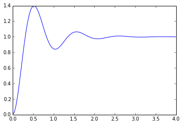
H = lti([wn*wn],[1, 2*zeta*wn, wn*wn])
t,y = H.step()
plt.plot(t,y)
print "max numerical value of step: %.6f" % np.max(y)
zeta = 0.279998
max numerical value of step: 1.399979
And here’s how to use lsim(). First we need to construct a test input. We could use the ratelimit() function I wrote earlier in this article, but I like closed-form solutions, and there is one for a rate-limited step. The reason I like closed-form solutions, rather than a numerical timeseries, is that we can write a waveform as a function of any time t, and evaluate it at any time we like, essentially giving us “infinite” precision in time, whereas a numerical timeseries is inherently discrete-time, even if the timesteps are variable. Chew on that for a while, and read on:
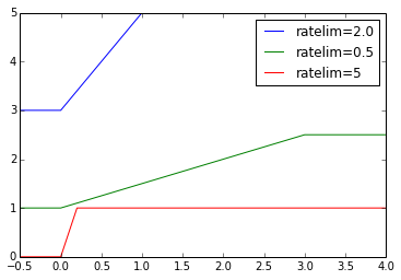
def ratelimitedstep(slewrate, initval=0.0, finalval=1.0):
    T_end = (finalval - initval) * 1.0 / slewrate
    A = (finalval-initval) / 2.0 / T_end
    B = (finalval+initval) / 2.0
    def f(t):
        return A*(np.abs(t) - np.abs(t-T_end)) + B
    return f

trange = [-0.5,4]
f2   = ratelimitedstep(2.0, initval=3.0, finalval = 5.0)
f0_5 = ratelimitedstep(0.5, initval=1.0, finalval = 2.5)
f5 = ratelimitedstep(5)
t = np.arange(trange[0],trange[1],0.01)
plt.plot(t,f2(t), t,f0_5(t),t,f5(t))
plt.xlim(trange)
plt.legend(('ratelim=2.0','ratelim=0.5','ratelim=5'),'best')
Now let’s put it all together:
t = np.arange(-1,5,0.001)
f = ratelimitedstep(2.0)
t2, y, _ = lsim(H,f(t),t)
tstep, ystep = H.step()
plt.plot(tstep,ystep,t2,y)
plt.plot(t,t>0,':',t,f(t),':')
plt.legend(('step response','response to ratelim step'),'best',fontsize=10)
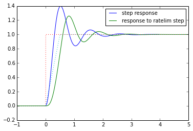
Tada! Now that’s interesting; the overshoot has been reduced. We’ll come back to this idea in a bit, but first let’s handle the other two approaches. Here’s an example using both the forward Euler, midpoint, and Runge-Kutta methods, as well as the step() function of scipy’s LTI objects:
import scipy.signal

def secondordersystem(wn,zeta,method):
    def fderiv(x,u):
        '''
        derivative function for 2nd-order system
        state variable x has two components:
        x[0] = output
        x[1] = derivative of output

        d2x/dt2 = (u-x)*wn^2 - 2*zeta*wn*(dx/dt)
        '''
        return (x[1], (u-x[0])*wn*wn - 2*zeta*wn*x[1])
    def project(x,dxdt,dt):
        '''project a state vector x forward by dx/dt * dt'''
        return (x[0]+dt*dxdt[0], x[1]+dt*dxdt[1])
    def solver(t,u,fderiv,stepper):
        x = (0,0)  # initial state
        tprev = t[0]
        uprev = u[0]
        for tval, uval in zip(t,u):
            dt = tval - tprev
            dxdt = stepper(fderiv,uprev,uval,x,dt)
            x = project(x,dxdt,dt)
            yield x[0]
            tprev = tval
            uprev = uval
    def forward_euler_step(fderiv,uprev,u,x,dt):
        return fderiv(x,u)
    def midpoint_method_step(fderiv,uprev,u,x,dt):
        dx1 = fderiv(x,u)
        xmid = project(x,dx1,dt/2)
        return fderiv(xmid,u)
    def runge_kutta_step(fderiv,uprev,u,x,dt):
        dx1 = fderiv(x,u)
        x1  = project(x,dx1,dt/2)
        dx2 = fderiv(x1,u)
        x2  = project(x,dx2,dt/2)
        dx3 = fderiv(x2,u)
        x3  = project(x,dx3,dt)
        dx4 = fderiv(x3,u)
        dxdt = ((dx1[0]+2*dx2[0]+2*dx3[0]+dx4[0])/6,
                (dx1[1]+2*dx2[1]+2*dx3[1]+dx4[1])/6)
        return dxdt
    if method == 'midpoint':
        stepper = midpoint_method_step
    elif method == 'euler':
        stepper = forward_euler_step
    elif method == 'runge':
        stepper = runge_kutta_step
    else:
        raise ValueError("method must be 'midpoint' or 'euler' or 'runge'")

    def sim(t,u):
        return np.array(list(solver(t,u,fderiv,stepper)))

    return sim

for timestep in [0.05, 0.01]:
    t = np.arange(-1,5,timestep)
    # add more points around the discontinuity
    t = np.union1d(t, np.arange(-5,5,0.01)*timestep)
    sos1 = secondordersystem(wn,zeta,'euler')
    sos2 = secondordersystem(wn,zeta,'midpoint')
    sos3 = secondordersystem(wn,zeta,'runge')
    u = (t>0)*1.0
    yeuler = sos1(t,u)
    ymid   = sos2(t,u)
    yrunge = sos3(t,u)

    def step2(H, t):
        '''make up for the fact that scipy step functions
        don't handle start times other than zero >:(
        '''
        return np.hstack((t[t<0]*0, H.step(T=t[t>=0])[1]))
    y = step2(H,t)
    plt.figure(figsize=(8,6))
    plt.subplot(4,1,1)
    plt.plot(t,yeuler,
             t,ymid,
             t,yrunge,
             t,y)
    plt.title('Simulation, timestep=%.3f' % timestep)
    for (i,approx) in enumerate([(yeuler,'Euler'),(ymid,'Midpoint'),(yrunge,'Runge-Kutta')]):
        plt.subplot(4,1,i+2)
        yapprox, approxname = approx
        plt.plot(t,yapprox-y)
        plt.ylabel('Error: %s' % approxname)
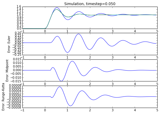
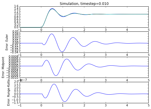
Woohoo! We get close to the expected value with step(), and the error term behaviors are what they should be, with Euler error being the largest, and midpoint and Runge-Kutta error decreasing more rapidly as a function of the timestep. There’s a subtlety here, though. I had to vary the timestep and decrease it near the discontinuity of the step input. Without this change, the timestep is constant, and when I tried this, the midpoint and Runge-Kutta solvers didn’t work much better than Euler, because the error introduced at the discontinuity persisted in the feedback state.
In addition to having to get all these details right, any of these approaches runs slower, since it happens within the Python environment, whereas lsim() and step() can use optimized implementations. So I’m going to abandon the manual approach and focus on the other two:
- The
lsim()approach is to create a rate-limited step waveform and uselsim()to find the response to it. - The
step()approach is to integrate the transfer function and use thestep()function to find two time-shifted ramp responses, which when subtracted yield the response to a ramp-limited step.
Let’s use both and see how close they get:
def rampresponse(H, t, t0):
    '''make up for the fact that scipy step functions
    don't handle start times other than zero >:(
    '''
    # Create a transfer function H * (1/s)
    # but we can't use 0 as the new coefficient because it
    # doesn't work with the step() code, so come close
    H_integrated = lti(H.num, np.hstack([H.den, 1e-9]))
    return np.hstack((t[t<t0]*0, H_integrated.step(T=t[t>=t0])[1]))

def ramplimstepresponse(H,ratelim,t):
    '''ramp-limited step with rate limit R =
    response to the difference between ramps r(t) - r(t-1/R)
    '''
    return (rampresponse(H,t,0) - rampresponse(H,t,1.0/ratelim))*ratelim

t = np.arange(-1,5,0.01)
ramprate = 2.0

# method 1: lsim()
f = ratelimitedstep(ramprate)
t1, y1, _ = lsim(H,f(t),t)
# method 2: step()
y2 = ramplimstepresponse(H,ramprate,t)

plt.subplot(211)
plt.plot(t,y1,t,y2)
plt.subplot(212)
plt.plot(t,y1-y2)
plt.ylabel('error')
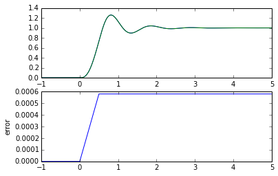
Which approach is better, and why do we see an error between the two? I don’t know which approach is better. I’m more confident in staying with lsim() becase it’s more straightforward and doesn’t involve hacks to create an approximate ramp response. I don’t know if the error is because of numerical issues in the calculations. Or maybe it has to do with the discontinuities in the beginning and end of the ramp, which combine with the inherent discrete time nature of the lsim() function.
That’s the end of our interlude.
Analyzing the overshoot
Let’s look at the overshoot in our system for different ramp-limited steps with the same ramp rate but different step sizes.
trange=[-0.5,6]
t = np.arange(trange[0],trange[1],0.01)
ratelim = 1.8
plt.figure(figsize=(8,6))
for usize in [0.5, 0.9, 0.95, 1.0, 2.0, 3.0, 4.0, 5.0, 6.0, 7.0, 8.0]:
    Trampend = usize/ratelim
    f = ratelimitedstep(ratelim/usize)
    u = f(t)*usize
    _, y, _ = lsim(H,u,t)
    # find maximum:
    # let's calculate this faster by using close-together points
    # that are in the neighborhood of the maximum
    i = np.argmax(y)
    ymax = y[i]
    tmax = t[i]
    t2 = np.union1d(t, tmax+np.arange(-0.1,0.1,0.0005))
    u2 = f(t2)*usize
    _, y2, _ = lsim(H,u2,t2)
    i = np.argmax(y2)
    ymax = y2[i]
    tmax = t2[i]
    print "step size=%5.2f, abs overshoot=%.4f" % (usize, ymax-usize)
    plt.plot(t,u,':',t2,y2,tmax,ymax,'.')
plt.xlim(trange)
plt.ylim(0,ymax*1.05)
step size= 0.50, abs overshoot=0.1757
step size= 0.90, abs overshoot=0.2331
step size= 0.95, abs overshoot=0.2334
step size= 1.00, abs overshoot=0.2323
step size= 2.00, abs overshoot=0.1427
step size= 3.00, abs overshoot=0.1755
step size= 4.00, abs overshoot=0.1638
step size= 5.00, abs overshoot=0.1677
step size= 6.00, abs overshoot=0.1664
step size= 7.00, abs overshoot=0.1668
step size= 8.00, abs overshoot=0.1667
(0, 8.5750331075081245)
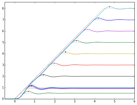
That’s interesting. I see three things to note:
-
The slew rate of the output can be greater than the slew rate of the input. (In fact, it turns out that the maximum output slew rate is 1.4 times the input slew rate, where the 1.4 comes from the step response overshoot of 0.4.) This means that if you want to use an underdamped system, and you want to keep the output slew rate below an absolute limit, you must derate that limit before using it as a slew rate limit of the system input.
-
Except for short steps comparable to the system response time, the absolute overshoot is about the same. It settles down to about 0.1667 for long steps. The peak overshoot is about 0.2334, which is 1.400 times as much. There’s that number again!
-
The output reaches a constant following error below the input. The following error for a unit ramp (with slope of 1) has nonzero steady-state error of \( 2\zeta/\omega_n \), and we’ll see why in that upcoming article on second order systems. So if we have a ramp rate of R, we should expect steady-state ramp error of \( 2\zeta R/\omega_n \).
If you go through a bunch of grungy algebra, the end result is that the overshoot OVSRL of a 2nd-order system with an input of a slew-rate limited step, if the ramp time is long, is proportional to the slew rate:
$$ OVSRL = \frac{SR}{\omega_n}e^{-\zeta\frac{\pi/2 + \sin^{-1}\zeta}{\sqrt{1-\zeta^2}}} $$
So we can decrease the overshoot by decreasing the slew rate. The overshoot of a step response with no slew rate limit is \( OV = e^{-\frac{\pi\zeta}{\sqrt{1-\zeta^2}}} \).
Just as a double-check:
def ovsr(wn,zeta,slewrate):
    return slewrate/wn*np.exp(-zeta*(np.pi/2 + np.arcsin(zeta))/np.sqrt(1-zeta**2))

ovsr(wn,zeta,ratelim)
0.16679199263977906
Bingo!
So, given ζ and ωn, we can predict the step reponse overshoot OV, we can predict the overshoot OVSRL for long ramp inputs, we can predict the maximum overshoot (= (1+OV)× OVSRL) for any ramp input, we can predict the maximum output slew rate (= (1+OV) × input slew rate) for any ramp input. How about that!
Method #2: Rate-limit the input using output feedback
Rate-limiting based purely on the input command is fairly straightforward, as we’ve seen. In systems with slow dynamics where the output takes a while to change, and our sensing of the output value is low-noise, there’s another method:
Limit the input command to within ± Δ of the output.
This actually uses the inherent dynamics of the output to help slew-rate limit the input. We found earlier that if we have an input ramp rate of R, we should expect steady-state ramp error, which is the steady-state difference between input and output during the ramp, of \( 2\zeta R/\omega_n \). The trick here is to work backwards: we start with that difference, so if we tweak the input to constrain the error between input and output to be at most Δ, then we can expect an input ramp rate R, and therefore choose \( \Delta = 2\zeta R/\omega_n \).
This approach also has the advantage that if the output gets “stuck” for some reason, the input command will wait for it.
In C this would look something like the function shown below. It’s actually identical to the first C function srlimit_update(), except that we feed in the system output rather than the previous input, and the value of delta is different.
int16_t srlimit_update2(int16_t x_raw_input,
                       int16_t system_output,
                       int16_t delta)
{
    // Constrain the input to be within some value "delta"
    // of the system output.

    // 1. Compute difference between raw input and output
    int32_t diff = (int32_t)x_raw_input - system_output;
    // 2. Limit this difference to within acceptable limits
    if (diff > delta)
        diff = delta;
    if (diff < -delta)
        diff = -delta;
    // 3. Apply the limited difference to
    //    compute the adjusted input.
    return system_output + (int16_t)diff;
}
We can try simulating this too, but to do so, we need to use the manual differential equation solver approach, since there is now feedback from the output to the input, and we therefore have a nonlinear system, which neither lsim() nor step() can help us with.
def secondordersystem_feedback(wn,zeta):
    '''2nd-order system simulator.
    u_limited = f(t, u_raw,x) is an input here.
    We use Runge-Kutta.
    '''
    def fderiv(x,u):
        '''
        derivative function for 2nd-order system
        state variable x has two components:
        x[0] = output
        x[1] = derivative of output

        d2x/dt2 = (u-x)*wn^2 - 2*zeta*wn*(dx/dt)
        '''
        return (x[1], (u-x[0])*wn*wn - 2*zeta*wn*x[1])
    def project(x,dxdt,dt):
        '''project a state vector x forward by dx/dt * dt'''
        return (x[0]+dt*dxdt[0], x[1]+dt*dxdt[1])
    def solver(t,u_raw,f,fderiv,stepper):
        x = (0,0)  # initial state
        tprev = t[0]
        uprev = 0
        for tval, urawval in zip(t,u_raw):
            dt = tval - tprev
            u = f(t,urawval,x[0])
            dxdt = stepper(fderiv,uprev,u,x,dt)
            x = project(x,dxdt,dt)
            yield (u,x[0],x[1])
            tprev = tval
            uprev = u
    def runge_kutta_step(fderiv,uprev,u,x,dt):
        dx1 = fderiv(x,u)
        x1  = project(x,dx1,dt/2)
        dx2 = fderiv(x1,u)
        x2  = project(x,dx2,dt/2)
        dx3 = fderiv(x2,u)
        x3  = project(x,dx3,dt)
        dx4 = fderiv(x3,u)
        dxdt = ((dx1[0]+2*dx2[0]+2*dx3[0]+dx4[0])/6,
                (dx1[1]+2*dx2[1]+2*dx3[1]+dx4[1])/6)
        return dxdt
    def sim(t,u_raw,f):
        '''returns a 3-column matrix:
        column 0 is the limited value u
        column 1 is the output x
        column 2 is the derivative dx/dt
        '''
        return np.array(list(solver(t,u_raw,f,fderiv,runge_kutta_step)))

    return sim

def slewrate_method2(delta):
    '''limit u to x +/- delta'''
    def f(t, u, x):
        if u > x+delta:
            u = x+delta
        elif u < x-delta:
            u = x-delta
        return u
    return f
Okay, let’s use it:
t = np.arange(-1,5,0.01)
# add more points around the discontinuity
t = np.union1d(t, np.arange(-5,5,0.01)*0.01)
u_raw = (t>0)*1.0

R = 0.8
delta = 2*zeta*R/wn
fslewer = slewrate_method2(delta)
sim = secondordersystem_feedback(wn,zeta)
ux = sim(t,u_raw,fslewer)
u = ux[:,0]
x = ux[:,1]
dxdt = ux[:,2]

import matplotlib.gridspec as gridspec
gs = gridspec.GridSpec(2, 1, height_ratios=[2,1])

fig = plt.figure(figsize=(8,6))
ax = plt.subplot(gs[0])
ax.fill_between(t, x+delta, x-delta, facecolor='gray', alpha=0.08)
ax.plot(t,u_raw,':',t,u,t,x)
ax.legend(('u_raw (raw input)','u (input)','x (output)'),'lower right')
ax.set_ylim(0,1.2)
ax.set_xlabel('time (s)')
ax.text(3,x[-1]-delta,'$\\Delta = %.3f$' % delta, fontsize=16)

ax2 = plt.subplot(gs[1])
ax2.plot(t,dxdt)
ax2.legend(('dx/dt',),'upper right')
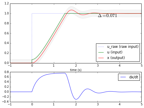
Woot! We controlled the maximum output slew rate to \( \pm R = 0.8 \) by limiting our input so that the difference between input and output is within \( \pm\Delta = 2R\zeta/\omega_n = 0.071 \). Now let’s compare and see what both methods look like:
trange = [-0.5,5]
t0 = np.arange(trange[0],trange[1],0.01)
R = 0.8

for t_unclamp in [0, 0.5]:
    # add more points around the discontinuity
    t = np.union1d(t0, t_unclamp + np.arange(-5,5,0.01)*0.01)
    u_raw = (t>0)*1.0

    # method 1 of slew-rate limiting:
    # derate to R/(1+overshoot)
    f = ratelimitedstep(R/1.400)
    u1 = f(t)
    u1_unclamped = u1 * (t>=t_unclamp)
    Hderiv = lti([wn*wn,0],[1,2*zeta*wn,wn*wn])
    _, x1, _ = lsim(H,u1_unclamped,t)
    _, dx1dt, _ = lsim(Hderiv,u1_unclamped,t)

    # method 2
    delta = 2*zeta*R/wn
    fslewer = slewrate_method2(delta)
    sim = secondordersystem_feedback(wn,zeta)
    tmask = t >= t_unclamp
    n_clamped = np.count_nonzero(~tmask)
    ux = sim(t[tmask],u_raw[tmask],fslewer)
    zeropad = np.zeros((n_clamped,3))
    zeropad[:,0] = np.clip(u_raw[~tmask],-delta,delta)
    ux = np.vstack((zeropad,ux))
    u2 = ux[:,0]
    x2 = ux[:,1]
    dx2dt = ux[:,2]

    import matplotlib.gridspec as gridspec
    gs = gridspec.GridSpec(2, 1, height_ratios=[2,1])

    fig = plt.figure(figsize=(8,6))
    ax = plt.subplot(gs[0])
    ax.fill_between(t, x2+delta, x2-delta, facecolor='gray', alpha=0.08)
    ax.plot(t,u_raw,':',
            t,u1,'black',t,x1,'red',
            t,u2,'blue',t,x2,'green')
    ax.legend(('u_raw (raw input)',
               'u_1 (input)','x_1 (output)',
               'u_2 (input)','x_2 (output)'),'lower right')
    ax.set_ylim(0,1.2)
    ax.set_xlabel('time (s)')
    ax.text(3,x[-1]-delta,'$\\Delta = %.3f$' % delta, fontsize=16)
    title = 'Comparison between two slew-rate limiting methods'
    if t_unclamp > 0:
        title += ',\n output unclamp at t=%.1f' % t_unclamp
    ax.set_title(title)
    ax.set_xlim(trange)

    ax2 = plt.subplot(gs[1])
    ax2.plot(t,dx1dt,t,dx2dt)
    ax2.set_xlim(trange)
    ax2.legend(('dx_1/dt','dx_2/dt'),'upper right')
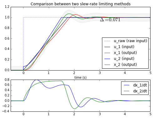
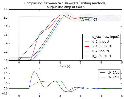
Okay, what are we looking at here?
The first graph shows that both methods keep the output slew rate within ±R. But the second method (constrain the input to the output ±Δ) finishes faster.
The second graph shows what happens if we clamp the output somehow to zero until t=0.5, and then unclamp it. The first method gets no feedback from the output and goes ahead and starts ramping up at t=0. At t=0.5, all of a sudden the output is unclamped and ZOOM! it has to catch up with the input ramp that has already started. In this case it settles earlier than the output of the second method. But we have failed to keep the output slew rate below the desired limit, which was the whole point of limiting the input. The second method works fine: it just waits patiently until the output starts to change, and then transitions smoothly towards its final value.
Which method is better?
I generally like the constrain-input-within-a-band-around-the-output approach better (method #2), if I know the output sensing is accurate and low-noise. If there is noise, a little bit of filtering (or even slew-rate limiting!) can reduce this noise to a reasonable value.
I suppose it’s possible to combine both methods, but there are some tricky corner cases where you have to give priority to one method over the other, for example if the raw input is pulled one way and a disturbance pulls the output another way, then the raw input and the output are far enough apart that you can’t satisfy both methods simultaneously.
Both of these methods have large portions of the initial rampup where the output rate of change is less than the allowed maximum. There’s probably yet another way to apply a slew rate to a system, by using feedback to push the input system as hard as we can, while keeping the output slew rate below the allowed maximum. But I’m skeptical whether it’s stable and robust and is not sensitive to noise.
Wrapup
Slew-rate limiting is a nonlinear behavior. In some systems it exists even though we don’t want it. In other systems, there’s not an inherent slew-rate limit, but we have good reason to add one: it keeps the system state within more well-behaved limits. Two well-known methods of slew-rate limiting are very similar. Given a raw input waveform \( u_0(t) \), we can do one of two things:
- Try to move the system input towards \( u_0 \), but constrain the input to within a band around the previous value of the input. (Feedforward slew rate limit.)
- Try to move the system input towards \( u_0 \), but constrain the input to within a band around the system output. (Feedback slew rate limit.)
In general the second method is better, as long as the output feedback sensing is accurate and low-noise.
We can use scipy.signal and its lti() and lsim() functions to try these methods out in Python. For the feedback slew rate limit technique, we have to use a differential equation solver to simulate it.
That’s all for now. One of these days I’ll get around to writing up my article on second-order systems, and you’ll hear more about overshoot.
© 2014 Jason M. Sachs, all rights reserved.


- Comments
- Write a Comment Select to add a comment
To post reply to a comment, click on the 'reply' button attached to each comment. To post a new comment (not a reply to a comment) check out the 'Write a Comment' tab at the top of the comments.
Please login (on the right) if you already have an account on this platform.
Otherwise, please use this form to register (free) an join one of the largest online community for Electrical/Embedded/DSP/FPGA/ML engineers:


