Linear Feedback Shift Registers for the Uninitiated, Part XVI: Reed-Solomon Error Correction

Jason Sachs●June 19, 2018

Last time, we talked about error correction and detection, covering some basics like Hamming distance, CRCs, and Hamming codes. If you are new to this topic, I would strongly suggest going back to read that article before this one.

This time we are going to cover Reed-Solomon codes. (I had meant to cover this topic in Part XV, but the article was getting to be too long, so I’ve split it roughly in half.) These are one of the workhorses of error-correction, and they are used in overwhelming abundance to correct short bursts of errors. We’ll see that encoding a message using Reed-Solomon is fairly simple, so easy that we can even do it in C on an embedded system.

We’re also going to talk about some performance metrics of error-correcting codes.

Reed-Solomon Codes

Reed-Solomon codes, like many other error-correcting codes, are parameterized. A Reed-Solomon $ (n,k) $ code, where $ n=2^m-1 $ and $ k=n-2t $, can correct up to $ t $ errors. They are not binary codes; each symbol must have $ 2^m $ possible values, and is typically an element of $ GF(2^m) $.

The Reed-Solomon codes with $ n=255 $ are very common, since then each symbol is an element of $ GF(2^8) $ and can be represented as a single byte. A $ (255, 247) $ RS code would be able to correct 4 errors, and a $ (255,223) $ RS code would be able to correct 16 errors, with each error being an arbitrary error in one transmitted symbol.

You may have noticed a pattern in some of the coding techniques discussed in the previous article:

If we compute the parity of a string of bits, and concatenate a parity bit, the resulting message has a parity of zero modulo 2
If we compute the checksum of a string of bytes, and concatenate a negated checksum, the resulting message has a checksum of zero modulo 256
If we compute the CRC of a message (with no initial/final bit flips), and concatenate the CRC, the resulting message has a remainder of zero modulo the CRC polynomial
If we compute parity bits of a Hamming code, and concatenate them to the data bits, the resulting message has a remainder of zero modulo the Hamming code polynomial

In all cases, we have this magic technique of taking data bits, using a division algorithm to compute the remainder, and concatenating the remainder, such that the resulting message has zero remainder. If we receive a message which does have a nonzero remainder, we can detect this, and in some cases use the nonzero remainder to determine where the errors occurred and correct them.

Parity and checksum are poor methods because they are unable to detect transpositions. It’s easy to cancel out a parity flip; it’s much harder to cancel out a CRC error by accidentally flipping another bit elsewhere.

What if there was an encoding algorithm that was somewhat similar to a checksum, in that it operated on a byte-by-byte basis, but had robustness to swapped bytes? Reed-Solomon is such an algorithm. And it amounts to doing the same thing as all the other linear coding techniques we’ve talked about to encode a message:

take data bits
use a polynomial division algorithm to compute a remainder
create a codeword by concatenating the data bits and the remainder bits
a valid codeword now has a zero remainder

In this article, I am going to describe Reed-Solomon encoding, but not the typical decoding methods, which are somewhat complicated, and include fancy-sounding steps like the Berlekamp-Massey algorithm (yes, this is the same one we saw in part VI, only it’s done in $ GF(2^m) $ instead of the binary $ GF(2) $ version), the Chien search, and the Forney algorithm. If you want to learn more, I would recommend reading the BBC white paper WHP031, in the list of references, which does go into just the right level of detail, and has lots of examples.

In addition to being more complicated to understand, decoding is also more computationally intensive. Reed-Solomon encoders are straightforward to implement in hardware — which we’ll see a bit later — and are simple to implement in software in an embedded system. Decoders are trickier, and you’d probably want something more powerful than an 8-bit microcontroller to execute them, or they’ll be very slow. The first use of Reed-Solomon in space communications was on the Voyager missions, where an encoder was included without certainty that the received signals could be decoded back on earth. From a NASA Tutorial on Reed-Solomon Error Correction Coding by William A. Geisel:

The Reed-Solomon (RS) codes have been finding widespread applications ever since the 1977 Voyager’s deep space communications system. At the time of Voyager’s launch, efficient encoders existed, but accurate decoding methods were not even available! The Jet Propulsion Laboratory (JPL) scientists and engineers gambled that by the time Voyager II would reach Uranus in 1986, decoding algorithms and equipment would be both available and perfected. They were correct! Voyager’s communications system was able to obtain a data rate of 21,600 bits per second from 2 billion miles away with a received signal energy 100 billion times weaker than a common wrist watch battery!

The statement “accurate decoding methods were not even available” in 1977 is a bit suspicious, although this general idea of faith-that-a-decoder-could-be-constructed is in several other accounts:

Lahmeyer, the sole engineer on the project, and his team of technicians and builders worked tirelessly to get the decoder working by the time Voyager reached Uranus. Otherwise, they would have had to slow down the rate of data received to decrease noise interference. “Each chip had to be hand wired,” Lahmeyer says. “Thankfully, we got it working on time.”

(Jefferson City Magazine, June 2015)

In order to make the extended mission to Uranus and Neptune possible, some new and never-before-tried technologies had to be designed into the spacecraft and novel new techniques for using the hardware to its fullest had to be validated for use. One notable requirement was the need to improve error correction coding of the data stream over the very inefficient method which had been used for all previous missions (and for the Voyagers at Jupiter and Saturn), because the much lower maximum data rates from Uranus and Neptune (due to distance) would have greatly compromised the number of pictures and other data that could have been obtained. A then-new and highly efficient data coding method called Reed-Solomon (RS) coding was planned for Voyager at Uranus, and the coding device was integrated into the spacecraft design. The problem was that although RS coding is easy to do and the encoding device was relatively simple to make, decoding the data after receipt on the ground is so mathematically intensive that no computer on Earth was able to handle the decoding task at the time Voyager was designed – or even launched. The increase of data throughput using the RS coder was about a factor of three over the old, standard Golay coding, so including the capability was considered highly worthwhile. It was assumed that a decoder could be developed by the time Voyager needed it at Uranus. Such was the case, and today RS coding is routinely used in CD players and many other common household electronic devices.

(Sirius Astronomer, August 2017)

Geisel probably meant “efficient” rather than “accurate”; decoding algorithms were well-known before a NASA report in 1978 which states

These codes were first described by I. S. Reed and G. Solomon in 1960. A systematic decoding algorithm was not discovered until 1968 by E. Berlekamp. Because of their complexity, the RS codes are not widely used except when no other codes are suitable.

Details of Reed-Solomon Encoding

At any rate, with Reed-Solomon, we have a polynomial, but instead of the coefficients being 0 or 1 like our usual polynomials in $ GF(2)[x] $, this time the coefficients are elements of $ GF(2^m) $. A byte-oriented Reed-Solomon encoding uses $ GF(2^8) $. The polynomial used in Reed-Solomon is usually written as $ g(x) $, the generator polynomial, with

$$g(x) = (x+\lambda^b)(x+\lambda^{b+1})(x+\lambda^{b+2})\ldots (x+\lambda^{b+n-k-1})$$

where $ \lambda $ is a primitive element of $ GF(2^m) $ and $ b $ is some constant, usually 0 or 1 or $ -t $. This means the polynomial’s roots are successive powers of $ \lambda $, and that makes the math work out just fine.

All we do is treat the message as a polynomial $ M(x) $, calculate a remainder $ r(x) = x^{n-k} M(x) \bmod g(x) $, and then concatenate it to the message; the resulting codeword $ C(x) = x^{n-k}M(x) + r(x) $, is guaranteed to be a multiple of the generator polynomial $ g(x) $. At the receiving end, we calculate $ C(x) \bmod g(x) $ and if it’s zero, everything’s great; otherwise we have to do some gory math, but this allows us to find and correct errors in up to $ t $ symbols.

That probably sounds rather abstract, so let’s work through an example.

Reed-Solomon in Python

We’re going to encode some messages using Reed-Solomon in two ways, first using the unireedsolomon library, and then from scratch using libgf2. If you’re going to use a library, you’ll need to be really careful; the library should be universal, meaning you can encode or decode any particular flavor of Reed-Solomon — like the CRC, there are many possible variants, and you need to be able to specify the polynomial of the Galois field used for each symbol, along with the generator element $ \lambda $ and the initial power $ b $. If anyone tells you they’re using the Reed-Solomon $ (255,223) $ code, they’re smoking something funny, because there’s more than one, and you need to know which particular variant in order to communicate properly.

There are two examples in the BBC white paper:

one using $ RS(15,11) $ for 4-bit symbols, with symbol field $ GF(2)[y]/(y^4 + y + 1) $; for the generator, $ \lambda = y = {\tt 2} $ and $ b=0 $, forming the generator polynomial

$$\begin{align} g(x) &= (x+1)(x+\lambda)(x+\lambda^2)(x+\lambda^3) \cr &= x^4 + \lambda^{12}x^3 + \lambda^{4}x^2 + x + \lambda^6 \cr &= x^4 + 15x^3 + 3x^2 + x + 12 \cr &= x^4 + {\tt F} x^3 + {\tt 3}x^2 + {\tt 1}x + {\tt 12} \end{align}$$

another using the DVB-T specification that uses $ RS(255,239) $ for 8-bit symbols, with symbol field $ GF(2)[y]/(y^8 + y^4 + y^3 + y^2 + 1) $ (hex representation 11d) and for the generator, $ \lambda = y = {\tt 2} $ and $ b=0 $, forming the generator polynomial

$$\begin{align} g(x) &= (x+1)(x+\lambda)(x+\lambda^2)(x+\lambda^3)\ldots(x+\lambda^{15}) \cr &= x^{16} + \lambda^{12}x^3 + \lambda^{4}x^2 + x + \lambda^6 \cr &= x^{16} + 59x^{15} + 13x^{14} + 104x^{13} + 189x^{12} + 68x^{11} + 209x^{10} + 30x^9 + 8x^8 \cr &\qquad + 163x^7 + 65x^6 + 41x^5 + 229x^4 + 98x^3 + 50x^2 + 36x + 59 \cr &= x^{16} + {\tt 3B} x^{15} + {\tt 0D}x^{14} + {\tt 68}x^{13} + {\tt BD}x^{12} + {\tt 44}x^{11} + {\tt d1}x^{10} + {\tt 1e}x^9 + {\tt 08}x^8\cr &\qquad + {\tt A3}x^7 + {\tt 41}x^6 + {\tt 29}x^5 + {\tt E5}x^4 + {\tt 62}x^3 + {\tt 32}x^2 + {\tt 24}x + {\tt 3B} \end{align}$$

In unireedsolomon, the RSCoder class is used, with these parameters:

c_exp — this is the number of bits per symbol, 4 and 8 for our two examples
prim — this is the symbol field polynomial, 0x13 and 0x11d for our two examples
generator — this is the generator element in the symbol field, 0x2 for both examples
fcr — this is the “first consecutive root” $ b $, with $ b=0 $ for both examples

You can verify the generator polynomial by encoding the message $ M(x) = 1 $, all zero symbols with a trailing one symbol at the end; this will create a codeword $ C(x) = x^{n-k} + r(x) = g(x) $.

Let’s do it!

import unireedsolomon as rs

def codeword_symbols(msg):
    return [ord(c) for c in msg]

def find_generator(rscoder):
    """ Returns the generator polynomial of an RSCoder class """
    msg = [0]*(rscoder.k - 1) + [1]
    degree = rscoder.n - rscoder.k
    codeword = rscoder.encode(msg)
    # look at the trailing elements of the codeword
    return codeword_symbols(codeword[(-degree-1):])

rs4 = rs.RSCoder(15,11,generator=2,prim=0x13,fcr=0,c_exp=4)
print "g4(x) = %s" % find_generator(rs4)

rs8 = rs.RSCoder(255,239,generator=2,prim=0x11d,fcr=0,c_exp=8)
print "g8(x) = %s" % find_generator(rs8)

g4(x) = [1, 15, 3, 1, 12]
g8(x) = [1, 59, 13, 104, 189, 68, 209, 30, 8, 163, 65, 41, 229, 98, 50, 36, 59]

Easy as pie!

Encoding messages is just a matter of using either a string (byte array) or a list of message symbols, and we get a string back by default. (You can use encode(msg, return_string=False) but then you get a bunch of GF2Int objects back rather than integer coefficients.)

(Warning: the unireedsolomon package uses a global singleton to manage Galois field arithmetic, so if you want to have multiple RSCoder objects out there, they’ll only work if they share the same field generator polynomial. This is why each time I want to switch back between the 4-bit and the 8-bit RSCoder, I have to create a new object, so that it reconfigures the way Galois field arithmetic works.)

The BBC white paper has a sample encoding only for the 4-bit $ RS(15,11) $ example, using $ [1,2,3,4,5,6,7,8,9,10,11] $ which produces remainder $ [3,3,12,12] $:

rs4 = rs.RSCoder(15,11,generator=2,prim=0x13,fcr=0,c_exp=4)
encmsg15 = codeword_symbols(rs4.encode([1,2,3,4,5,6,7,8,9,10,11]))
print "RS(15,11) encoded example message from BBC WHP031:\n", encmsg15

RS(15,11) encoded example message from BBC WHP031:
[1, 2, 3, 4, 5, 6, 7, 8, 9, 10, 11, 3, 3, 12, 12]

The real fun begins when we can start encoding actual messages, like Ernie, you have a banana in your ear! Since this has length 37, let’s use a shortened version of the code, $ RS(53,37) $.

Mama’s Little Baby Loves Shortnin’, Shortnin’, Mama’s Little Baby Loves Shortnin’ Bread

Oh, we haven’t talked about shortened codes yet — this is where we just omit the initial symbols in a codeword, and both transmitter and receiver agree treat them as implied zeros. An eight-bit $ RS(53,37) $ transmitter encodes as codeword polynomials of degree 52, and the receiver just zero-extends them to degree 254 (with 202 implied zero bytes added at the beginning) for the purposes of decoding just like any other $ RS(255,239) $ code.

rs8s = rs.RSCoder(53,37,generator=2,prim=0x11d,fcr=0,c_exp=8)
msg = 'Ernie, you have a banana in your ear!'
codeword = rs8s.encode(msg)
print ('codeword=%r' % codeword)
remainder = codeword[-16:]
print ('remainder(hex) = %s' % remainder.encode('hex'))

codeword='Ernie, you have a banana in your ear!U,\xa3\xb4d\x00:R\xc4P\x11\xf4n\x0f\xea\x9b'
remainder(hex) = 552ca3b464003a52c45011f46e0fea9b

That binary stuff after the message is the remainder. Now we can decode all sorts of messages with errors:

for init_msg in [
    'Ernie, you have a banana in your ear!',
    'Billy! You have a banana in your ear!',
    'Arnie! You have a potato in your ear!',
    'Eddie? You hate a banana in your car?',
    '01234567ou have a banana in your ear!',
    '012345678u have a banana in your ear!',
]:
    decoded_msg, decoded_remainder = rs8s.decode(init_msg+remainder)
    print "%s -> %s" % (init_msg, decoded_msg)

Ernie, you have a banana in your ear! -> Ernie, you have a banana in your ear!
Billy! You have a banana in your ear! -> Ernie, you have a banana in your ear!
Arnie! You have a potato in your ear! -> Ernie, you have a banana in your ear!
Eddie? You hate a banana in your car? -> Ernie, you have a banana in your ear!
01234567ou have a banana in your ear! -> Ernie, you have a banana in your ear!

---------------------------------------------------------------------------
RSCodecError                              Traceback (most recent call last)
 in ()
      7     '012345678u have a banana in your ear!',
      8 ]:
----> 9     decoded_msg, decoded_remainder = rs8s.decode(init_msg+remainder)
     10     print "%s -> %s" % (init_msg, decoded_msg)

/Users/jmsachs/anaconda/lib/python2.7/site-packages/unireedsolomon/rs.pyc in decode(self, r, nostrip, k, erasures_pos, only_erasures, return_string)
    321         # being the rightmost byte
    322         # X is a corresponding array of GF(2^8) values where X_i = alpha^(j_i)
--> 323         X, j = self._chien_search(sigma)
    324 
    325         # Sanity check: Cannot guarantee correct decoding of more than n-k errata (Singleton Bound, n-k being the minimum distance), and we cannot even check if it's correct (the syndrome will always be all 0 if we try to decode above the bound), thus it's better to just return the input as-is.

/Users/jmsachs/anaconda/lib/python2.7/site-packages/unireedsolomon/rs.pyc in _chien_search(self, sigma)
    822         errs_nb = len(sigma) - 1 # compute the exact number of errors/errata that this error locator should find
    823         if len(j) != errs_nb:
--> 824             raise RSCodecError("Too many (or few) errors found by Chien Search for the errata locator polynomial!")
    825 
    826         return X, j

RSCodecError: Too many (or few) errors found by Chien Search for the errata locator polynomial!

This last message failed to decode because there were 9 errors and $ RS(53,37) $ or $ RS(255,239) $ can only correct 8 errors.

But if there are few enough errors, Reed-Solomon will fix them all.

Why does it work?

The reason why Reed-Solomon encoding and decoding works is a bit hard to grasp. There are quite a few good explanations of how encoding and decoding works, my favorite being the BBC whitepaper, but none of them really dwells upon why it works. We can handwave about redundancy and the mysteriousness of finite fields spreading that redundancy evenly throughout the remainder bits, or a spectral interpretation of the parity-check matrix where the roots of the generator polynomial can be considered as “frequencies”, but I don’t have a good explanation. Here’s the best I can do:

Let’s say we have some number of errors where the locations are known. This is called an erasure, in contrast to a true error, where the location is not known ahead of time. Think of a bunch of symbols on a piece of paper, and some idiot erases one of them or spills vegetable soup, and you’ve lost one of the symbols, but you know where it is. The message received could be 45 72 6e 69 65 2c 20 ?? 6f 75 where the ?? represents an erasure. Of course, binary computers don’t have a way to compute arithmetic on ??, so what we would do instead is just pick an arbitrary pattern like 00 or 42 to replace the erasure, and mark its position (in this case, byte 7) for later processing.

Anyway, in a Reed-Solomon code, the error values are linearly independent. This is really the key here. We can have up to $ 2t $ erasures (as opposed to $ t $ true errors) and still maintain this linear independence property. Linear independence means that for a system of equations, there is only one solution. An error in bytes 3 and 28, for example, can’t be mistaken for an error in bytes 9 and 14. Once you exceed the maximum number of errors or erasures, the linear independence property falls apart and there are many possible ways to correct received errors, so we can’t be sure which is the right one.

To get a little more technical: we have a transmitted coded message $ C_t(x) = x^{n-k}M(x) + r(x) $ where $ M(x) $ is the unencoded message and $ r(x) $ is the remainder modulo the generator polynomial $ g(x) $, and a received message $ C_r(x) = C_t(x) + e(x) $ where the error polynomial $ e(x) $ represents the difference between transmitted and received messages. The receiver can compute $ e(x) \bmod g(x) $ by calculating the remainder $ C_r(x) \bmod g(x) $. If there are no errors, then $ e(x) \bmod g(x) = 0 $. With erasures, we know the locations of the errors. Let’s say we had $ n=255 $, $ 2t=16 $, and we had three errors at known locations $ i_1, i_2, $ and $ i_3, $ in which case $ e(x) = e_{i_1}x^{i_1} + e_{i_2}x^{i_2} + e_{i_3}x^{i_3} $. These terms $ e_{i_1}x^{i_1}, e_{i_2}x^{i_2}, $ etc. are the error values that form a linear independent set. For example, if the original message had 42 in byte 13, but we received 59 instead, then the error coefficient in that location would be 42 + 59 = 1B, so $ i_1 = 13 $ and the error value would be $ {\tt 1B}x^{13} $.

What the algebra of finite fields assures us, is that if we have a suitable choice of generator polynomial $ g(x) $ of degree $ 2t $ — and the one used for Reed-Solomon, $ g(x) = \prod\limits_{i=0}^{2t-1}(x-\lambda^{b+i}) $, is suitable — then any selection of up to $ 2t $ distinct powers of $ x $ from $ x^0 $ to $ x^{n-1} $ are linearly independent. If $ 2t = 16 $, for example, then we cannot write $ x^{15} = ax^{13} + bx^{8} + c $ for some choices of $ a,b,c $ — otherwise it would mean that $ x^{15}, x^{13}, x^8, $ and $ 1 $ do not form a linearly independent set. This means that if we have up to $ 2t $ erasures at known locations, then we can figure out the coefficients at each location, and find the unknown values.

In our 3-erasures example above, if $ 2t=16, i_1 = 13, i_2 = 8, i_3 = 0 $, then we have a really easy case. All the errors are in positions below the degree of the remainder, which means all the errors are in the remainder, and the message symbols arrived intact. In this case, the error polynomial looks like $ e(x) = e_{13}x^{13} + e_8x^8 + e_0 $ for some error coefficients $ e_{13}, e_8, e_0 $ in $ GF(256) $. The received remainder $ e(x) \bmod g(x) = e(x) $ and we can just find the error coefficients directly.

On the other hand, let’s say we knew the errors were in positions $ i_1 = 200, i_2 = 180, i_3 = 105 $. In this case we could calculate $ x^{200} \bmod g(x) $, $ x^{180} \bmod g(x) $, and $ x^{105} \bmod g(x) $. These each have a bunch of coefficients from degree 0 to 15, but we know that the received remainder $ e(x) \bmod g(x) $ must be a linear combination of the three polynomials, $ e_{200}x^{200} + e_{180}x^{180} + e_{105}x^{105} \bmod g(x) $ and we could solve for $ e_{200} $, $ e_{180} $, and $ e_{105} $ using linear algebra.

A similar situation applies if we have true errors where we don’t know their positions ahead of time. In this case we can correct only $ t $ errors, but the algebra works out so that we can write $ 2t $ equations with $ 2t $ unknowns (an error location and value for each of the $ t $ errors) and solve them.

All we need is for someone to prove this linear independence property. That part I won’t be able to explain intuitively. If you look at the typical decoder algorithms, they will show constructively how to find the unique solution, but not why it works. Reed-Solomon decoders make use of the so-called “key equation”; for Euclidean algorithm decoders (as opposed to Berlekamp-Massey decoders), the key equation is $ \Omega(x) = S(x)\Lambda(x) \bmod x^{2t} $ and you’re supposed to know what that means and how to use it… sigh. A bit of blind faith sometimes helps.

Which is why I won’t have anything more to say on decoding. Read the BBC whitepaper.

Reed-Solomon Encoding in `libgf2`

We don’t have to use the unireedsolomon library as a black box. We can do the encoding step in libgf2 using libgf2.lfsr.PolyRingOverField. This is a helper class that the undecimate() function uses. I talked a little bit about this in part XI, along with some of the details of this “two-variable” kind of mathematical thing, a polynomial ring over a finite field. Let’s forget about the abstract math for now, and just start computing. The PolyRingOverField just defines a particular arithmetic of polynomials, represented as lists of coefficients in ascending order (so $ x^2 + 2 $ is represented as [2, 0, 1]):

from libgf2.gf2 import GF2QuotientRing, GF2Polynomial
from libgf2.lfsr import PolyRingOverField
import numpy as np

f16 = GF2QuotientRing(0x13)
f256 = GF2QuotientRing(0x11d)
rsprof16  = PolyRingOverField(f16)
rsprof256 = PolyRingOverField(f256)

p1 = [1,4]
p2 = [2,8]
rsprof256.mul(p1, p2)

[2, 0, 32]

def compute_generator_polynomial(rsprof, elementfield, k):
    el = 1
    g = [1]
    n = (1 << elementfield.degree) - 1 
    for _ in xrange(n-k):
        g = rsprof.mul(g, [el, 1])
        el = elementfield.mulraw(el, 2)
    return g

g16 = compute_generator_polynomial(rsprof16, f16, 11)
g256 = compute_generator_polynomial(rsprof256, f256, 239)
print "generator polynomials (in ascending order of coefficients)"
print "RS(15,11):    g16=", g16
print "RS(255,239): g256=", g256

generator polynomials (in ascending order of coefficients)
RS(15,11):    g16= [12, 1, 3, 15, 1]
RS(255,239): g256= [59, 36, 50, 98, 229, 41, 65, 163, 8, 30, 209, 68, 189, 104, 13, 59, 1]

Now, to encode a message, we just have to convert binary data to polynomials and then take the remainder $ \bmod g(x) $:

print "BBC WHP031 example for RS(15,11):"
msg_bbc = [1,2,3,4,5,6,7,8,9,10,11]
msgpoly = [0]*4 + [c for c in reversed(msg_bbc)]
print "message=%r" % msg_bbc
q,r = rsprof16.divmod(msgpoly, g16)
print "remainder=", r

print "\nReal-world example for RS(255,239):"
print "message=%r" % msg
msgpoly = [0]*16 + [ord(c) for c in reversed(msg)]
q,r = rsprof256.divmod(msgpoly, g256)
print "remainder=", r
print "in hex: ", ''.join('%02x' % b for b in reversed(r))
print "remainder calculated earlier:\n         %s" % remainder.encode('hex')

BBC WHP031 example for RS(15,11):
message=[1, 2, 3, 4, 5, 6, 7, 8, 9, 10, 11]
remainder= [12, 12, 3, 3]

Real-world example for RS(255,239):
message='Ernie, you have a banana in your ear!'
remainder= [155, 234, 15, 110, 244, 17, 80, 196, 82, 58, 0, 100, 180, 163, 44, 85]
in hex:  552ca3b464003a52c45011f46e0fea9b
remainder calculated earlier:
         552ca3b464003a52c45011f46e0fea9b

See how easy that is?

Well… you probably didn’t, because PolyRingOverField hides the implementation of the abstract algebra. We can make the encoding step even easier to understand if we take the perspective of an LFSR.

Chocolate Strawberry Peach Vanilla Banana Pistachio Peppermint Lemon Orange Butterscotch

We can handle Reed-Solomon encoding in either software or hardware (and at least the remainder-calculating part of the decoder) using LFSRs. Now, we have to loosen up what we mean by an LFSR. So far, all the LFSRs have dealt directly with binary bits, and each shift cell either has a tap, or doesn’t, depending on the coefficients of the polynomial associated with the LFSR. For Reed-Solomon, the units of computation are elements of $ GF(256) $, represented as 8-bit bytes for a particular degree-8 primitive polynomial. So the shift cells, instead of containing bits, will contain bytes, and the taps will change from simple taps to multipliers over $ GF(256) $. (This gets a little hairy in hardware, but it’s not that bad.) A 10-byte LFSR over $ GF(256) $ implementing Reed-Solomon encoding would look something like this:

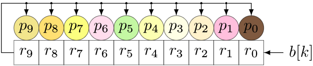
We would feed the bytes $ b[k] $ of the message in at the right; bytes $ r_0 $ through $ r_9 $ represent a remainder, and coefficients $ p_0 $ through $ p_9 $ represent the non-leading coefficients of the RS code’s generator polynomial. In this case, we would use a 10th-degree generator polynomial with a leading coefficient 1.

For each new byte, we do two things:

Shift all cells left, shifting in one byte of the message
Take the byte shifted out, and multiply it by the generator polynomial, then add (XOR) with the contents of the shift register.

We also have to remember to do this another $ n-k $ times (the length of the shift register) to cover the $ x^{n-k} $ factor. (Remember, we’re trying to calculate $ r(x) = x^{n-k}M(x) $.)

f256 = GF2QuotientRing(0x11d)

def rsencode_lfsr1(field, message, gtaps, remainder_only=False):
    """ encode a message in Reed-Solomon using LFSR
    field: symbol field
    message: string of bytes
    gtaps: generator polynomial coefficients, in ascending order
    remainder_only: whether to return the remainder only
    """
    glength = len(gtaps)
    remainder = np.zeros(glength, np.int)
    for char in message + '\0'*glength:
        remainder = np.roll(remainder, 1)
        out = remainder[0]
        remainder[0] = ord(char)
        for k, c in enumerate(gtaps):
            remainder[k] ^= field.mulraw(c, out)
    remainder = ''.join(chr(b) for b in reversed(remainder))
    return remainder if remainder_only else message+remainder

print rsencode_lfsr1(f256, msg, g[:-1], remainder_only=True).encode('hex')
print "calculated earlier:"
print remainder.encode('hex')

552ca3b464003a52c45011f46e0fea9b
calculated earlier:
552ca3b464003a52c45011f46e0fea9b

That worked, but we still have to handle multiplication in the symbol field, which is annoying and cumbersome for embedded processors. There are two table-driven methods that make this step easier, relegating the finite field stuff either to initialization steps only, or something that can be done at design time if you’re willing to generate a table in source code. (For example, using Python to generate the table coefficients in C.)

Also we have that call to np.roll(), which is too high-level for a language like C, so let’s look at things from this low-level, table-driven approach.

One table method is to take the generator polynomial and multiply it by each of the 256 possible coefficients, so that we get a table of 256 × $ n-k $ bytes.

def rsencode_lfsr2_table(field, gtaps):
    """
    Create a table for Reed-Solomon encoding using a field
    This time the taps are in *descending* order
    """
    return [[field.mulraw(b,c) for c in gtaps] for b in xrange(256)]

def rsencode_lfsr2(table, message, remainder_only=False):
    """ encode a message in Reed-Solomon using LFSR
    table: table[i][j] is the multiplication of 
             generator coefficient of x^{n-k-1-j} by incoming byte i
    message: string of bytes
    remainder_only: whether to return the remainder only
    """
    glength = len(table[0])
    remainder = [0]*glength
    for char in message + '\0'*glength:
        out = remainder[0]
        table_row = table[out]
        for k in xrange(glength-1):
            remainder[k] = remainder[k+1] ^ table_row[k]
        remainder[glength-1] = ord(char) ^ table_row[glength-1]
    remainder = ''.join(chr(b) for b in remainder)
    return remainder if remainder_only else message+remainder

table = rsencode_lfsr2_table(f256, g[-2::-1])
print "table:"
for k, row in enumerate(table):
    print "%02x: %s" % (k, ' '.join('%02x' % c for c in row))

table:
00: 00 00 00 00 00 00 00 00 00 00 00 00 00 00 00 00
01: 3b 0d 68 bd 44 d1 1e 08 a3 41 29 e5 62 32 24 3b
02: 76 1a d0 67 88 bf 3c 10 5b 82 52 d7 c4 64 48 76
03: 4d 17 b8 da cc 6e 22 18 f8 c3 7b 32 a6 56 6c 4d
04: ec 34 bd ce 0d 63 78 20 b6 19 a4 b3 95 c8 90 ec
05: d7 39 d5 73 49 b2 66 28 15 58 8d 56 f7 fa b4 d7
06: 9a 2e 6d a9 85 dc 44 30 ed 9b f6 64 51 ac d8 9a
07: a1 23 05 14 c1 0d 5a 38 4e da df 81 33 9e fc a1
08: c5 68 67 81 1a c6 f0 40 71 32 55 7b 37 8d 3d c5
09: fe 65 0f 3c 5e 17 ee 48 d2 73 7c 9e 55 bf 19 fe
0a: b3 72 b7 e6 92 79 cc 50 2a b0 07 ac f3 e9 75 b3
0b: 88 7f df 5b d6 a8 d2 58 89 f1 2e 49 91 db 51 88
0c: 29 5c da 4f 17 a5 88 60 c7 2b f1 c8 a2 45 ad 29
0d: 12 51 b2 f2 53 74 96 68 64 6a d8 2d c0 77 89 12
0e: 5f 46 0a 28 9f 1a b4 70 9c a9 a3 1f 66 21 e5 5f
0f: 64 4b 62 95 db cb aa 78 3f e8 8a fa 04 13 c1 64
10: 97 d0 ce 1f 34 91 fd 80 e2 64 aa f6 6e 07 7a 97
11: ac dd a6 a2 70 40 e3 88 41 25 83 13 0c 35 5e ac
12: e1 ca 1e 78 bc 2e c1 90 b9 e6 f8 21 aa 63 32 e1
13: da c7 76 c5 f8 ff df 98 1a a7 d1 c4 c8 51 16 da
14: 7b e4 73 d1 39 f2 85 a0 54 7d 0e 45 fb cf ea 7b
15: 40 e9 1b 6c 7d 23 9b a8 f7 3c 27 a0 99 fd ce 40
16: 0d fe a3 b6 b1 4d b9 b0 0f ff 5c 92 3f ab a2 0d
17: 36 f3 cb 0b f5 9c a7 b8 ac be 75 77 5d 99 86 36
18: 52 b8 a9 9e 2e 57 0d c0 93 56 ff 8d 59 8a 47 52
19: 69 b5 c1 23 6a 86 13 c8 30 17 d6 68 3b b8 63 69
1a: 24 a2 79 f9 a6 e8 31 d0 c8 d4 ad 5a 9d ee 0f 24
1b: 1f af 11 44 e2 39 2f d8 6b 95 84 bf ff dc 2b 1f
1c: be 8c 14 50 23 34 75 e0 25 4f 5b 3e cc 42 d7 be
1d: 85 81 7c ed 67 e5 6b e8 86 0e 72 db ae 70 f3 85
1e: c8 96 c4 37 ab 8b 49 f0 7e cd 09 e9 08 26 9f c8
1f: f3 9b ac 8a ef 5a 57 f8 dd 8c 20 0c 6a 14 bb f3
20: 33 bd 81 3e 68 3f e7 1d d9 c8 49 f1 dc 0e f4 33
21: 08 b0 e9 83 2c ee f9 15 7a 89 60 14 be 3c d0 08
22: 45 a7 51 59 e0 80 db 0d 82 4a 1b 26 18 6a bc 45
23: 7e aa 39 e4 a4 51 c5 05 21 0b 32 c3 7a 58 98 7e
24: df 89 3c f0 65 5c 9f 3d 6f d1 ed 42 49 c6 64 df
25: e4 84 54 4d 21 8d 81 35 cc 90 c4 a7 2b f4 40 e4
26: a9 93 ec 97 ed e3 a3 2d 34 53 bf 95 8d a2 2c a9
27: 92 9e 84 2a a9 32 bd 25 97 12 96 70 ef 90 08 92
28: f6 d5 e6 bf 72 f9 17 5d a8 fa 1c 8a eb 83 c9 f6
29: cd d8 8e 02 36 28 09 55 0b bb 35 6f 89 b1 ed cd
2a: 80 cf 36 d8 fa 46 2b 4d f3 78 4e 5d 2f e7 81 80
2b: bb c2 5e 65 be 97 35 45 50 39 67 b8 4d d5 a5 bb
2c: 1a e1 5b 71 7f 9a 6f 7d 1e e3 b8 39 7e 4b 59 1a
2d: 21 ec 33 cc 3b 4b 71 75 bd a2 91 dc 1c 79 7d 21
2e: 6c fb 8b 16 f7 25 53 6d 45 61 ea ee ba 2f 11 6c
2f: 57 f6 e3 ab b3 f4 4d 65 e6 20 c3 0b d8 1d 35 57
30: a4 6d 4f 21 5c ae 1a 9d 3b ac e3 07 b2 09 8e a4
31: 9f 60 27 9c 18 7f 04 95 98 ed ca e2 d0 3b aa 9f
32: d2 77 9f 46 d4 11 26 8d 60 2e b1 d0 76 6d c6 d2
33: e9 7a f7 fb 90 c0 38 85 c3 6f 98 35 14 5f e2 e9
34: 48 59 f2 ef 51 cd 62 bd 8d b5 47 b4 27 c1 1e 48
35: 73 54 9a 52 15 1c 7c b5 2e f4 6e 51 45 f3 3a 73
36: 3e 43 22 88 d9 72 5e ad d6 37 15 63 e3 a5 56 3e
37: 05 4e 4a 35 9d a3 40 a5 75 76 3c 86 81 97 72 05
38: 61 05 28 a0 46 68 ea dd 4a 9e b6 7c 85 84 b3 61
39: 5a 08 40 1d 02 b9 f4 d5 e9 df 9f 99 e7 b6 97 5a
3a: 17 1f f8 c7 ce d7 d6 cd 11 1c e4 ab 41 e0 fb 17
3b: 2c 12 90 7a 8a 06 c8 c5 b2 5d cd 4e 23 d2 df 2c
3c: 8d 31 95 6e 4b 0b 92 fd fc 87 12 cf 10 4c 23 8d
3d: b6 3c fd d3 0f da 8c f5 5f c6 3b 2a 72 7e 07 b6
3e: fb 2b 45 09 c3 b4 ae ed a7 05 40 18 d4 28 6b fb
3f: c0 26 2d b4 87 65 b0 e5 04 44 69 fd b6 1a 4f c0
40: 66 67 1f 7c d0 7e d3 3a af 8d 92 ff a5 1c f5 66
41: 5d 6a 77 c1 94 af cd 32 0c cc bb 1a c7 2e d1 5d
42: 10 7d cf 1b 58 c1 ef 2a f4 0f c0 28 61 78 bd 10
43: 2b 70 a7 a6 1c 10 f1 22 57 4e e9 cd 03 4a 99 2b
44: 8a 53 a2 b2 dd 1d ab 1a 19 94 36 4c 30 d4 65 8a
45: b1 5e ca 0f 99 cc b5 12 ba d5 1f a9 52 e6 41 b1
46: fc 49 72 d5 55 a2 97 0a 42 16 64 9b f4 b0 2d fc
47: c7 44 1a 68 11 73 89 02 e1 57 4d 7e 96 82 09 c7
48: a3 0f 78 fd ca b8 23 7a de bf c7 84 92 91 c8 a3
49: 98 02 10 40 8e 69 3d 72 7d fe ee 61 f0 a3 ec 98
4a: d5 15 a8 9a 42 07 1f 6a 85 3d 95 53 56 f5 80 d5
4b: ee 18 c0 27 06 d6 01 62 26 7c bc b6 34 c7 a4 ee
4c: 4f 3b c5 33 c7 db 5b 5a 68 a6 63 37 07 59 58 4f
4d: 74 36 ad 8e 83 0a 45 52 cb e7 4a d2 65 6b 7c 74
4e: 39 21 15 54 4f 64 67 4a 33 24 31 e0 c3 3d 10 39
4f: 02 2c 7d e9 0b b5 79 42 90 65 18 05 a1 0f 34 02
50: f1 b7 d1 63 e4 ef 2e ba 4d e9 38 09 cb 1b 8f f1
51: ca ba b9 de a0 3e 30 b2 ee a8 11 ec a9 29 ab ca
52: 87 ad 01 04 6c 50 12 aa 16 6b 6a de 0f 7f c7 87
53: bc a0 69 b9 28 81 0c a2 b5 2a 43 3b 6d 4d e3 bc
54: 1d 83 6c ad e9 8c 56 9a fb f0 9c ba 5e d3 1f 1d
55: 26 8e 04 10 ad 5d 48 92 58 b1 b5 5f 3c e1 3b 26
56: 6b 99 bc ca 61 33 6a 8a a0 72 ce 6d 9a b7 57 6b
57: 50 94 d4 77 25 e2 74 82 03 33 e7 88 f8 85 73 50
58: 34 df b6 e2 fe 29 de fa 3c db 6d 72 fc 96 b2 34
59: 0f d2 de 5f ba f8 c0 f2 9f 9a 44 97 9e a4 96 0f
5a: 42 c5 66 85 76 96 e2 ea 67 59 3f a5 38 f2 fa 42
5b: 79 c8 0e 38 32 47 fc e2 c4 18 16 40 5a c0 de 79
5c: d8 eb 0b 2c f3 4a a6 da 8a c2 c9 c1 69 5e 22 d8
5d: e3 e6 63 91 b7 9b b8 d2 29 83 e0 24 0b 6c 06 e3
5e: ae f1 db 4b 7b f5 9a ca d1 40 9b 16 ad 3a 6a ae
5f: 95 fc b3 f6 3f 24 84 c2 72 01 b2 f3 cf 08 4e 95
60: 55 da 9e 42 b8 41 34 27 76 45 db 0e 79 12 01 55
61: 6e d7 f6 ff fc 90 2a 2f d5 04 f2 eb 1b 20 25 6e
62: 23 c0 4e 25 30 fe 08 37 2d c7 89 d9 bd 76 49 23
63: 18 cd 26 98 74 2f 16 3f 8e 86 a0 3c df 44 6d 18
64: b9 ee 23 8c b5 22 4c 07 c0 5c 7f bd ec da 91 b9
65: 82 e3 4b 31 f1 f3 52 0f 63 1d 56 58 8e e8 b5 82
66: cf f4 f3 eb 3d 9d 70 17 9b de 2d 6a 28 be d9 cf
67: f4 f9 9b 56 79 4c 6e 1f 38 9f 04 8f 4a 8c fd f4
68: 90 b2 f9 c3 a2 87 c4 67 07 77 8e 75 4e 9f 3c 90
69: ab bf 91 7e e6 56 da 6f a4 36 a7 90 2c ad 18 ab
6a: e6 a8 29 a4 2a 38 f8 77 5c f5 dc a2 8a fb 74 e6
6b: dd a5 41 19 6e e9 e6 7f ff b4 f5 47 e8 c9 50 dd
6c: 7c 86 44 0d af e4 bc 47 b1 6e 2a c6 db 57 ac 7c
6d: 47 8b 2c b0 eb 35 a2 4f 12 2f 03 23 b9 65 88 47
6e: 0a 9c 94 6a 27 5b 80 57 ea ec 78 11 1f 33 e4 0a
6f: 31 91 fc d7 63 8a 9e 5f 49 ad 51 f4 7d 01 c0 31
70: c2 0a 50 5d 8c d0 c9 a7 94 21 71 f8 17 15 7b c2
71: f9 07 38 e0 c8 01 d7 af 37 60 58 1d 75 27 5f f9
72: b4 10 80 3a 04 6f f5 b7 cf a3 23 2f d3 71 33 b4
73: 8f 1d e8 87 40 be eb bf 6c e2 0a ca b1 43 17 8f
74: 2e 3e ed 93 81 b3 b1 87 22 38 d5 4b 82 dd eb 2e
75: 15 33 85 2e c5 62 af 8f 81 79 fc ae e0 ef cf 15
76: 58 24 3d f4 09 0c 8d 97 79 ba 87 9c 46 b9 a3 58
77: 63 29 55 49 4d dd 93 9f da fb ae 79 24 8b 87 63
78: 07 62 37 dc 96 16 39 e7 e5 13 24 83 20 98 46 07
79: 3c 6f 5f 61 d2 c7 27 ef 46 52 0d 66 42 aa 62 3c
7a: 71 78 e7 bb 1e a9 05 f7 be 91 76 54 e4 fc 0e 71
7b: 4a 75 8f 06 5a 78 1b ff 1d d0 5f b1 86 ce 2a 4a
7c: eb 56 8a 12 9b 75 41 c7 53 0a 80 30 b5 50 d6 eb
7d: d0 5b e2 af df a4 5f cf f0 4b a9 d5 d7 62 f2 d0
7e: 9d 4c 5a 75 13 ca 7d d7 08 88 d2 e7 71 34 9e 9d
7f: a6 41 32 c8 57 1b 63 df ab c9 fb 02 13 06 ba a6
80: cc ce 3e f8 bd fc bb 74 43 07 39 e3 57 38 f7 cc
81: f7 c3 56 45 f9 2d a5 7c e0 46 10 06 35 0a d3 f7
82: ba d4 ee 9f 35 43 87 64 18 85 6b 34 93 5c bf ba
83: 81 d9 86 22 71 92 99 6c bb c4 42 d1 f1 6e 9b 81
84: 20 fa 83 36 b0 9f c3 54 f5 1e 9d 50 c2 f0 67 20
85: 1b f7 eb 8b f4 4e dd 5c 56 5f b4 b5 a0 c2 43 1b
86: 56 e0 53 51 38 20 ff 44 ae 9c cf 87 06 94 2f 56
87: 6d ed 3b ec 7c f1 e1 4c 0d dd e6 62 64 a6 0b 6d
88: 09 a6 59 79 a7 3a 4b 34 32 35 6c 98 60 b5 ca 09
89: 32 ab 31 c4 e3 eb 55 3c 91 74 45 7d 02 87 ee 32
8a: 7f bc 89 1e 2f 85 77 24 69 b7 3e 4f a4 d1 82 7f
8b: 44 b1 e1 a3 6b 54 69 2c ca f6 17 aa c6 e3 a6 44
8c: e5 92 e4 b7 aa 59 33 14 84 2c c8 2b f5 7d 5a e5
8d: de 9f 8c 0a ee 88 2d 1c 27 6d e1 ce 97 4f 7e de
8e: 93 88 34 d0 22 e6 0f 04 df ae 9a fc 31 19 12 93
8f: a8 85 5c 6d 66 37 11 0c 7c ef b3 19 53 2b 36 a8
90: 5b 1e f0 e7 89 6d 46 f4 a1 63 93 15 39 3f 8d 5b
91: 60 13 98 5a cd bc 58 fc 02 22 ba f0 5b 0d a9 60
92: 2d 04 20 80 01 d2 7a e4 fa e1 c1 c2 fd 5b c5 2d
93: 16 09 48 3d 45 03 64 ec 59 a0 e8 27 9f 69 e1 16
94: b7 2a 4d 29 84 0e 3e d4 17 7a 37 a6 ac f7 1d b7
95: 8c 27 25 94 c0 df 20 dc b4 3b 1e 43 ce c5 39 8c
96: c1 30 9d 4e 0c b1 02 c4 4c f8 65 71 68 93 55 c1
97: fa 3d f5 f3 48 60 1c cc ef b9 4c 94 0a a1 71 fa
98: 9e 76 97 66 93 ab b6 b4 d0 51 c6 6e 0e b2 b0 9e
99: a5 7b ff db d7 7a a8 bc 73 10 ef 8b 6c 80 94 a5
9a: e8 6c 47 01 1b 14 8a a4 8b d3 94 b9 ca d6 f8 e8
9b: d3 61 2f bc 5f c5 94 ac 28 92 bd 5c a8 e4 dc d3
9c: 72 42 2a a8 9e c8 ce 94 66 48 62 dd 9b 7a 20 72
9d: 49 4f 42 15 da 19 d0 9c c5 09 4b 38 f9 48 04 49
9e: 04 58 fa cf 16 77 f2 84 3d ca 30 0a 5f 1e 68 04
9f: 3f 55 92 72 52 a6 ec 8c 9e 8b 19 ef 3d 2c 4c 3f
a0: ff 73 bf c6 d5 c3 5c 69 9a cf 70 12 8b 36 03 ff
a1: c4 7e d7 7b 91 12 42 61 39 8e 59 f7 e9 04 27 c4
a2: 89 69 6f a1 5d 7c 60 79 c1 4d 22 c5 4f 52 4b 89
a3: b2 64 07 1c 19 ad 7e 71 62 0c 0b 20 2d 60 6f b2
a4: 13 47 02 08 d8 a0 24 49 2c d6 d4 a1 1e fe 93 13
a5: 28 4a 6a b5 9c 71 3a 41 8f 97 fd 44 7c cc b7 28
a6: 65 5d d2 6f 50 1f 18 59 77 54 86 76 da 9a db 65
a7: 5e 50 ba d2 14 ce 06 51 d4 15 af 93 b8 a8 ff 5e
a8: 3a 1b d8 47 cf 05 ac 29 eb fd 25 69 bc bb 3e 3a
a9: 01 16 b0 fa 8b d4 b2 21 48 bc 0c 8c de 89 1a 01
aa: 4c 01 08 20 47 ba 90 39 b0 7f 77 be 78 df 76 4c
ab: 77 0c 60 9d 03 6b 8e 31 13 3e 5e 5b 1a ed 52 77
ac: d6 2f 65 89 c2 66 d4 09 5d e4 81 da 29 73 ae d6
ad: ed 22 0d 34 86 b7 ca 01 fe a5 a8 3f 4b 41 8a ed
ae: a0 35 b5 ee 4a d9 e8 19 06 66 d3 0d ed 17 e6 a0
af: 9b 38 dd 53 0e 08 f6 11 a5 27 fa e8 8f 25 c2 9b
b0: 68 a3 71 d9 e1 52 a1 e9 78 ab da e4 e5 31 79 68
b1: 53 ae 19 64 a5 83 bf e1 db ea f3 01 87 03 5d 53
b2: 1e b9 a1 be 69 ed 9d f9 23 29 88 33 21 55 31 1e
b3: 25 b4 c9 03 2d 3c 83 f1 80 68 a1 d6 43 67 15 25
b4: 84 97 cc 17 ec 31 d9 c9 ce b2 7e 57 70 f9 e9 84
b5: bf 9a a4 aa a8 e0 c7 c1 6d f3 57 b2 12 cb cd bf
b6: f2 8d 1c 70 64 8e e5 d9 95 30 2c 80 b4 9d a1 f2
b7: c9 80 74 cd 20 5f fb d1 36 71 05 65 d6 af 85 c9
b8: ad cb 16 58 fb 94 51 a9 09 99 8f 9f d2 bc 44 ad
b9: 96 c6 7e e5 bf 45 4f a1 aa d8 a6 7a b0 8e 60 96
ba: db d1 c6 3f 73 2b 6d b9 52 1b dd 48 16 d8 0c db
bb: e0 dc ae 82 37 fa 73 b1 f1 5a f4 ad 74 ea 28 e0
bc: 41 ff ab 96 f6 f7 29 89 bf 80 2b 2c 47 74 d4 41
bd: 7a f2 c3 2b b2 26 37 81 1c c1 02 c9 25 46 f0 7a
be: 37 e5 7b f1 7e 48 15 99 e4 02 79 fb 83 10 9c 37
bf: 0c e8 13 4c 3a 99 0b 91 47 43 50 1e e1 22 b8 0c
c0: aa a9 21 84 6d 82 68 4e ec 8a ab 1c f2 24 02 aa
c1: 91 a4 49 39 29 53 76 46 4f cb 82 f9 90 16 26 91
c2: dc b3 f1 e3 e5 3d 54 5e b7 08 f9 cb 36 40 4a dc
c3: e7 be 99 5e a1 ec 4a 56 14 49 d0 2e 54 72 6e e7
c4: 46 9d 9c 4a 60 e1 10 6e 5a 93 0f af 67 ec 92 46
c5: 7d 90 f4 f7 24 30 0e 66 f9 d2 26 4a 05 de b6 7d
c6: 30 87 4c 2d e8 5e 2c 7e 01 11 5d 78 a3 88 da 30
c7: 0b 8a 24 90 ac 8f 32 76 a2 50 74 9d c1 ba fe 0b
c8: 6f c1 46 05 77 44 98 0e 9d b8 fe 67 c5 a9 3f 6f
c9: 54 cc 2e b8 33 95 86 06 3e f9 d7 82 a7 9b 1b 54
ca: 19 db 96 62 ff fb a4 1e c6 3a ac b0 01 cd 77 19
cb: 22 d6 fe df bb 2a ba 16 65 7b 85 55 63 ff 53 22
cc: 83 f5 fb cb 7a 27 e0 2e 2b a1 5a d4 50 61 af 83
cd: b8 f8 93 76 3e f6 fe 26 88 e0 73 31 32 53 8b b8
ce: f5 ef 2b ac f2 98 dc 3e 70 23 08 03 94 05 e7 f5
cf: ce e2 43 11 b6 49 c2 36 d3 62 21 e6 f6 37 c3 ce
d0: 3d 79 ef 9b 59 13 95 ce 0e ee 01 ea 9c 23 78 3d
d1: 06 74 87 26 1d c2 8b c6 ad af 28 0f fe 11 5c 06
d2: 4b 63 3f fc d1 ac a9 de 55 6c 53 3d 58 47 30 4b
d3: 70 6e 57 41 95 7d b7 d6 f6 2d 7a d8 3a 75 14 70
d4: d1 4d 52 55 54 70 ed ee b8 f7 a5 59 09 eb e8 d1
d5: ea 40 3a e8 10 a1 f3 e6 1b b6 8c bc 6b d9 cc ea
d6: a7 57 82 32 dc cf d1 fe e3 75 f7 8e cd 8f a0 a7
d7: 9c 5a ea 8f 98 1e cf f6 40 34 de 6b af bd 84 9c
d8: f8 11 88 1a 43 d5 65 8e 7f dc 54 91 ab ae 45 f8
d9: c3 1c e0 a7 07 04 7b 86 dc 9d 7d 74 c9 9c 61 c3
da: 8e 0b 58 7d cb 6a 59 9e 24 5e 06 46 6f ca 0d 8e
db: b5 06 30 c0 8f bb 47 96 87 1f 2f a3 0d f8 29 b5
dc: 14 25 35 d4 4e b6 1d ae c9 c5 f0 22 3e 66 d5 14
dd: 2f 28 5d 69 0a 67 03 a6 6a 84 d9 c7 5c 54 f1 2f
de: 62 3f e5 b3 c6 09 21 be 92 47 a2 f5 fa 02 9d 62
df: 59 32 8d 0e 82 d8 3f b6 31 06 8b 10 98 30 b9 59
e0: 99 14 a0 ba 05 bd 8f 53 35 42 e2 ed 2e 2a f6 99
e1: a2 19 c8 07 41 6c 91 5b 96 03 cb 08 4c 18 d2 a2
e2: ef 0e 70 dd 8d 02 b3 43 6e c0 b0 3a ea 4e be ef
e3: d4 03 18 60 c9 d3 ad 4b cd 81 99 df 88 7c 9a d4
e4: 75 20 1d 74 08 de f7 73 83 5b 46 5e bb e2 66 75
e5: 4e 2d 75 c9 4c 0f e9 7b 20 1a 6f bb d9 d0 42 4e
e6: 03 3a cd 13 80 61 cb 63 d8 d9 14 89 7f 86 2e 03
e7: 38 37 a5 ae c4 b0 d5 6b 7b 98 3d 6c 1d b4 0a 38
e8: 5c 7c c7 3b 1f 7b 7f 13 44 70 b7 96 19 a7 cb 5c
e9: 67 71 af 86 5b aa 61 1b e7 31 9e 73 7b 95 ef 67
ea: 2a 66 17 5c 97 c4 43 03 1f f2 e5 41 dd c3 83 2a
eb: 11 6b 7f e1 d3 15 5d 0b bc b3 cc a4 bf f1 a7 11
ec: b0 48 7a f5 12 18 07 33 f2 69 13 25 8c 6f 5b b0
ed: 8b 45 12 48 56 c9 19 3b 51 28 3a c0 ee 5d 7f 8b
ee: c6 52 aa 92 9a a7 3b 23 a9 eb 41 f2 48 0b 13 c6
ef: fd 5f c2 2f de 76 25 2b 0a aa 68 17 2a 39 37 fd
f0: 0e c4 6e a5 31 2c 72 d3 d7 26 48 1b 40 2d 8c 0e
f1: 35 c9 06 18 75 fd 6c db 74 67 61 fe 22 1f a8 35
f2: 78 de be c2 b9 93 4e c3 8c a4 1a cc 84 49 c4 78
f3: 43 d3 d6 7f fd 42 50 cb 2f e5 33 29 e6 7b e0 43
f4: e2 f0 d3 6b 3c 4f 0a f3 61 3f ec a8 d5 e5 1c e2
f5: d9 fd bb d6 78 9e 14 fb c2 7e c5 4d b7 d7 38 d9
f6: 94 ea 03 0c b4 f0 36 e3 3a bd be 7f 11 81 54 94
f7: af e7 6b b1 f0 21 28 eb 99 fc 97 9a 73 b3 70 af
f8: cb ac 09 24 2b ea 82 93 a6 14 1d 60 77 a0 b1 cb
f9: f0 a1 61 99 6f 3b 9c 9b 05 55 34 85 15 92 95 f0
fa: bd b6 d9 43 a3 55 be 83 fd 96 4f b7 b3 c4 f9 bd
fb: 86 bb b1 fe e7 84 a0 8b 5e d7 66 52 d1 f6 dd 86
fc: 27 98 b4 ea 26 89 fa b3 10 0d b9 d3 e2 68 21 27
fd: 1c 95 dc 57 62 58 e4 bb b3 4c 90 36 80 5a 05 1c
fe: 51 82 64 8d ae 36 c6 a3 4b 8f eb 04 26 0c 69 51
ff: 6a 8f 0c 30 ea e7 d8 ab e8 ce c2 e1 44 3e 4d 6a

print rsencode_lfsr2(table, msg, remainder_only=True).encode('hex')
print "calculated earlier:"
print remainder.encode('hex')

552ca3b464003a52c45011f46e0fea9b
calculated earlier:
552ca3b464003a52c45011f46e0fea9b

Alternatively, if none of the generating polynomial’s coefficients are zero, we can just represent these coefficients as powers of a generating element of a field, and then store log and antilog tables of $ x^n $ in the symbol field. These are each a smaller table of length 256 (with one dummy entry) and they remove all dependencies on doing arithmetic in the symbol field.

def rsencode_lfsr3_table(field_polynomial):
    """
    Create log and antilog tables for Reed-Solomon encoding using a field
    This just uses powers of x^n.
    """
    log = [0] * 256
    antilog = [0] * 256
    c = 1
    for k in xrange(255):
        antilog[k] = c
        log[c] = k
        c <<= 1
        cxor = c ^ field_polynomial
        if cxor < c:
            c = cxor
    return log, antilog

def rsencode_lfsr3(log, antilog, gpowers, message, remainder_only=False):
    """ encode a message in Reed-Solomon using LFSR
    log, antilog: tables for log and antilog: log[x^i] = i, antilog[i] = x^i
    gpowers: generator polynomial coefficients x^i, represented as i, in descending order
    message: string of bytes
    remainder_only: whether to return the remainder only
    """
    glength = len(gpowers)
    remainder = [0]*glength
    for char in message + '\0'*glength:
        out = remainder[0]
        if out == 0:
            # No multiplication. Just shift.
            for k in xrange(glength-1):
                remainder[k] = remainder[k+1]
            remainder[glength-1] = ord(char)
        else:
            outp = log[out]
            for k in xrange(glength-1):
                j = gpowers[k] + outp
                if j >= 255:
                    j -= 255
                remainder[k] = remainder[k+1] ^ antilog[j]
            j = gpowers[glength-1] + outp
            if j >= 255:
                j -= 255
            remainder[glength-1] = ord(char) ^ antilog[j]
    remainder = ''.join(chr(b) for b in remainder)
    return remainder if remainder_only else message+remainder

log, antilog = rsencode_lfsr3_table(f256.coeffs)
for (name, table) in [('log',log),('antilog',antilog)]:
    print "%s:" % name
    for k in xrange(0,256,16):
        print "%03d-%03d: %s" % (k,k+15,
                ' '.join('%02x' % c for c in table[k:k+16]))

log:
000-015: 00 00 01 19 02 32 1a c6 03 df 33 ee 1b 68 c7 4b
016-031: 04 64 e0 0e 34 8d ef 81 1c c1 69 f8 c8 08 4c 71
032-047: 05 8a 65 2f e1 24 0f 21 35 93 8e da f0 12 82 45
048-063: 1d b5 c2 7d 6a 27 f9 b9 c9 9a 09 78 4d e4 72 a6
064-079: 06 bf 8b 62 66 dd 30 fd e2 98 25 b3 10 91 22 88
080-095: 36 d0 94 ce 8f 96 db bd f1 d2 13 5c 83 38 46 40
096-111: 1e 42 b6 a3 c3 48 7e 6e 6b 3a 28 54 fa 85 ba 3d
112-127: ca 5e 9b 9f 0a 15 79 2b 4e d4 e5 ac 73 f3 a7 57
128-143: 07 70 c0 f7 8c 80 63 0d 67 4a de ed 31 c5 fe 18
144-159: e3 a5 99 77 26 b8 b4 7c 11 44 92 d9 23 20 89 2e
160-175: 37 3f d1 5b 95 bc cf cd 90 87 97 b2 dc fc be 61
176-191: f2 56 d3 ab 14 2a 5d 9e 84 3c 39 53 47 6d 41 a2
192-207: 1f 2d 43 d8 b7 7b a4 76 c4 17 49 ec 7f 0c 6f f6
208-223: 6c a1 3b 52 29 9d 55 aa fb 60 86 b1 bb cc 3e 5a
224-239: cb 59 5f b0 9c a9 a0 51 0b f5 16 eb 7a 75 2c d7
240-255: 4f ae d5 e9 e6 e7 ad e8 74 d6 f4 ea a8 50 58 af
antilog:
000-015: 01 02 04 08 10 20 40 80 1d 3a 74 e8 cd 87 13 26
016-031: 4c 98 2d 5a b4 75 ea c9 8f 03 06 0c 18 30 60 c0
032-047: 9d 27 4e 9c 25 4a 94 35 6a d4 b5 77 ee c1 9f 23
048-063: 46 8c 05 0a 14 28 50 a0 5d ba 69 d2 b9 6f de a1
064-079: 5f be 61 c2 99 2f 5e bc 65 ca 89 0f 1e 3c 78 f0
080-095: fd e7 d3 bb 6b d6 b1 7f fe e1 df a3 5b b6 71 e2
096-111: d9 af 43 86 11 22 44 88 0d 1a 34 68 d0 bd 67 ce
112-127: 81 1f 3e 7c f8 ed c7 93 3b 76 ec c5 97 33 66 cc
128-143: 85 17 2e 5c b8 6d da a9 4f 9e 21 42 84 15 2a 54
144-159: a8 4d 9a 29 52 a4 55 aa 49 92 39 72 e4 d5 b7 73
160-175: e6 d1 bf 63 c6 91 3f 7e fc e5 d7 b3 7b f6 f1 ff
176-191: e3 db ab 4b 96 31 62 c4 95 37 6e dc a5 57 ae 41
192-207: 82 19 32 64 c8 8d 07 0e 1c 38 70 e0 dd a7 53 a6
208-223: 51 a2 59 b2 79 f2 f9 ef c3 9b 2b 56 ac 45 8a 09
224-239: 12 24 48 90 3d 7a f4 f5 f7 f3 fb eb cb 8b 0b 16
240-255: 2c 58 b0 7d fa e9 cf 83 1b 36 6c d8 ad 47 8e 00

gpowers = [log[c] for c in g[-2::-1]]
print "generator polynomial coefficient indices: ", gpowers
print "remainder:"
print rsencode_lfsr3(log, antilog, gpowers, msg, remainder_only=True).encode('hex')
print "calculated earlier:"
print remainder.encode('hex')

generator polynomial coefficient indices:  [120, 104, 107, 109, 102, 161, 76, 3, 91, 191, 147, 169, 182, 194, 225, 120]
remainder:
552ca3b464003a52c45011f46e0fea9b
calculated earlier:
552ca3b464003a52c45011f46e0fea9b

There. It’s very simple; the hardest thing here is making sure you get the coefficients in the right order. You wouldn’t want to get those the wrong way around.

C Implementation

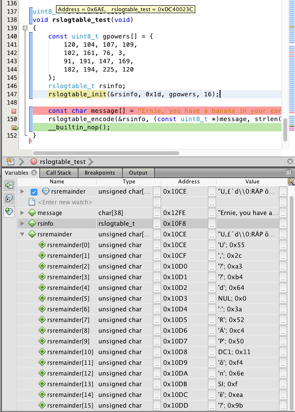
I tested a C implementation using XC16 and the MPLAB X debugger:

""" C code for reed-solomon.c:
/*
 *
 * Copyright 2018 Jason M. Sachs
 *
 * Licensed under the Apache License, Version 2.0 (the "License");
 * you may not use this file except in compliance with the License.
 * You may obtain a copy of the License at
 *
 *   http://www.apache.org/licenses/LICENSE-2.0
 *
 * Unless required by applicable law or agreed to in writing, software
 * distributed under the License is distributed on an "AS IS" BASIS,
 * WITHOUT WARRANTIES OR CONDITIONS OF ANY KIND, either express or implied.
 * See the License for the specific language governing permissions and
 * limitations under the License.
 */

#include <stdint.h>
#include <stddef.h>
#include <string.h>

/**
 * Reed-Solomon log-table-based implementation
 */
typedef struct {
    uint8_t log[256];
    uint8_t antilog[256];
    uint8_t symbol_polynomial;
    const uint8_t *gpowers;
    uint8_t generator_degree;
} rslogtable_t;


/**
 * Initialize log table
 * 
 * @param ptables - points to log tables
 * @param symbol_polynomial: lower 8 bits of symbol polynomial
 *         (for example, 0x1d for 0x11d = x^8 + x^4 + x^3 + x^2 + 1
 * @param gpowers - points to generator polynomial coefficients,
 *         except for the leading monomial,
 *         in descending order, expressed as powers of x in the symbol field.
 *         This requires all generator polynomial coefficients to be nonzero.
 * @param generator_degree - degree of the generator polynomial,
 *         which is also the length of the gpowers array.
 */
void rslogtable_init(
    rslogtable_t *ptables, 
    uint8_t symbol_polynomial,
    const uint8_t *gpowers,
    uint8_t generator_degree
)
{
    ptables->symbol_polynomial = symbol_polynomial;
    ptables->gpowers = gpowers;
    ptables->generator_degree = generator_degree;
    
    int k;
    uint8_t c = 1;
    for (k = 0; k < 255; ++k)
    {
        ptables->antilog[k] = c;
        ptables->log[c] = k;
        if (c >> 7)
        {
            c <<= 1;
            c ^= symbol_polynomial;
        }
        else
        {
            c <<= 1;
        }
    }
    ptables->log[0] = 0;
    ptables->antilog[255] = 0;
}

/**
 * Encode a message
 * 
 * @param ptables - pointer to table-based lookup info
 * @param pmessage - message to be encoded 
 * @param message_length - length of the message
 * @param premainder - buffer which will be filled in with the remainder.
 *     This must have a size equal to ptables->generator_degree
 */
void rslogtable_encode(
    const rslogtable_t *ptables,
    const uint8_t *pmessage,
    size_t message_length,
    uint8_t *premainder 
)
{
    int i, j, k, n;
    int highbyte;
    const int t2 = ptables->generator_degree;
    const int lastindex = t2-1;
    
    // Zero out the remainder
    for (i = 0; i < t2; ++i)
    {
        premainder[i] = 0;
    }
    
    n = message_length + t2;
    for (i = 0; i < n; ++i)
    {
        uint8_t c = (i < message_length) ? pmessage[i] : 0;
        highbyte = premainder[0];
        if (highbyte == 0)
        {
            // No multiplication, just a simple shift
            for (k = 0; k < lastindex; ++k)
            {
                premainder[k] = premainder[k+1];
            }
            premainder[lastindex] = c;
        }
        else
        {
            uint8_t log_highbyte = ptables->log[highbyte];
            for (k = 0; k < lastindex; ++k)
            {
                j = ptables->gpowers[k] + (int)log_highbyte;
                if (j >= 255)
                    j -= 255;
                premainder[k] = premainder[k+1] ^ ptables->antilog[j];
            }
            j = ptables->gpowers[lastindex] + (int)log_highbyte;
            if (j >= 255)
                j -= 255;
            premainder[lastindex] = c ^ ptables->antilog[j];
        }
    }
}

uint8_t rsremainder[16];
void rslogtable_test(void)
{
    const uint8_t gpowers[] = {
        120, 104, 107, 109, 
        102, 161, 76, 3, 
        91, 191, 147, 169,
        182, 194, 225, 120
    };
    rslogtable_t rsinfo;
    rslogtable_init(&rsinfo, 0x1d, gpowers, 16);
    
    const char message[] = "Ernie, you have a banana in your ear!";
    rslogtable_encode(&rsinfo, (const uint8_t *)message, strlen(message), rsremainder);
    __builtin_nop();
}
""";

It worked as expected:

Again, this is only the encoder, but remember the asymmetry here:

encoder = cheap resource-limited processor
decoder = desktop PC CPU

And we can still do error correction!

Is It Worth It?

Is encoding worth the effort?

Wait. We got all the way through Part XV and well into this article, you say, and he’s asking is it worth it?!

Yes, that’s the question. We got a benefit, namely the ability to detect and sometimes even correct errors, but it has a cost. We have to send extra information, and that uses up part of the available communications bandwidth. And we had to add some complexity. Is it a net gain?

There are at least two ways of looking at this cost-benefit tradeoff, and it depends on what the constraints are.

The first way of analyzing cost-benefits is to consider a situation where we’re given a transmitter/receiver pair, and all we have control over is the digital part of the system that handles the bits that are sent. Error correcting codes like Reed-Solomon give us the ability to lower the error rate substantially — and we’ll calculate this in just a minute — with only a slight decrease in transmission rate. A $ (255, 239) $ Reed-Solomon code lets us correct up to 8 errors in each block of 255 bytes, with 93.7% of the transmission capacity of the uncoded channel. The encoding complexity cost is minimal, and the decoding cost is small enough to merit use of Reed-Solomon decoders in higher-end embedded systems or in desktop computers.

The second way of analyzing cost-benefits is to consider a situation where we have control over the transmitter energy, as well as the digital encoding/decoding mechanisms. We can lower the error rate by using an error-correcting code, or we can increase the transmitter energy to improve the signal-to-noise ratio. The Shannon-Hartley theorem, which says channel capacity $ C \leq B \log_2 (1+\frac{S}{N}) $, can help us quantitatively compare those possibilities. The standard metric is $ E_b/N_0 $ in decibels, so let’s try to frame things in terms of it. First we have to understand what it is.

One common assumption in communications is an additive Gaussian white noise (AWGN) channel, which has some amount of noise $ N_0 $ per unit bandwidth. This is why oscilloscopes let you limit the bandwidth; if you don’t need it, it reduces the noise level. In any case, if we have an integrate-and-dump receiver, where we integrate our received signal, and every $ T $ seconds we sample the integrator value, divide by $ T $ to compute an average value over the interval, and reset the integrator, then the received noise can be modeled as a Gaussian random variable with zero mean and variance of $ \sigma_N^2 = \frac{N_0}{2T} $. (This can be computed from $ \sigma_N^2 = \frac{N_0}{2}\int_{-\infty}^{\infty}\left|h(t)\right|^2\, dt $ with $ h(t) $ of the integrate-and-dump filter being a unit rectangular pulse of duration $ T $ and height $ 1/T $.)

The signal waveform has some energy $ E_b $ per bit. Consider a raw binary pulse signal $ x(t) = \pm A $ for a duration of $ T $ seconds for each bit, with $ +A $ representing a binary 1 and $ -A $ representing a binary 0. If we compute $ E_b = \int_{-\infty}^{\infty}\left|x(t)\right|^2\, dt $ we get $ E_b = A^2T $. The integrate-and-dump receiver outputs a 1 if its output sample is positive, and 0 if its output sample is negative. We get a bit flip if the received noise is less than $ -A $ for a transmitted 1 bit, or greater than $ A $ for a transmitted 0 bit. This probability is just the Q-function evaluated at $ Q(A/\sigma_n) = Q(\sqrt{A^2/\sigma_n{}^2}) = Q(\sqrt{(E_b/T)/(N_0/2T)}) = Q(\sqrt{2E_b/N_0}). $

In other words, if we know how bits are represented as signals, we can determine the probability of a bit error just by knowing what $ E_b/N_0 $ is.

Let’s graph it!

Bit Error Rate Calculations Are the Bane of My Existence

Just one quick aside: this section showing bit error rate graphs was a beastly thing to manage. Don’t worry about the Python code, or how the calculations work, unless you want to enter this quagmire. Otherwise, just look at the pretty pictures, and my descriptions of how to interpret them.

As I was saying, let’s graph it!

import numpy as np
import pandas as pd
import matplotlib.pyplot as plt
%matplotlib inline
import scipy.stats

def Q(x):
    return scipy.stats.norm.cdf(-x)

def Qinv(x):
    return -scipy.stats.norm.ppf(x)

ebno_db = np.arange(-6,12,0.01)
ebno = 10**(ebno_db/10)
# Decibels are often confusing.
# dB = 10 log10 x  if x is measured in energy
# dB = 20 log10 x  if x is measured in amplitude. 

plt.semilogy(ebno_db, Q(np.sqrt(2*ebno)))
plt.ylabel('Bit error rate',fontsize=12)
plt.xlabel('$E_b/N_0$ (dB)',fontsize=12)
plt.grid('on')
plt.title('Bit error rate for raw binary pulses in AWGN channel\n'
          +'with integrate-and-dump receiver');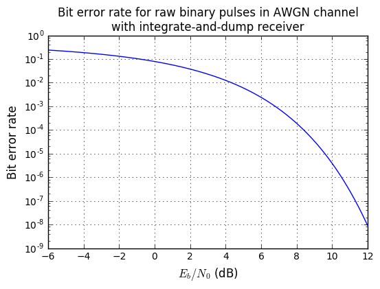

If we have a nice healthy noise margin of 12dB for $ E_b/N_0 $, then the bit error rate is $ 9.0\times 10^{-9} $, or one error in 110 million. Again, this is just raw binary pulses using an integrate-and-dump receiver. More complex signal shaping techniques like quadrature amplitude modulation can make better use of available spectrum. But that’s an article for someone else to write.

With an $ E_b/N_0 $ ratio of 1 (that’s 0dB), probability of a bit error is around 0.079, or about one in 12. Lousy. You want a lower error rate? Put more energy into the signal, or make sure there’s less energy in noise.

Okay, now suppose we use a Hamming (7,4) code. Let’s say, for example, that the raw bit error rate is 0.01, which occurs at about $ E_b/N_0 \approx 4.3 $dB. With the Hamming (7,4) code, we can correct one error, so there are a few cases to consider for an upper bound that is conservative and assumes some worst-case conditions:

There were no received bit errors. Probability of this is $ (1-0.01)^7 \approx 0.932065. $ The receiver will output 4 correct output bits, and there are no errors after decoding
There was one received bit error, in one of the seven codeword bits. Probability of this is $ 7\cdot 0.01\cdot(1-0.01)^6 \approx 0.065904. $ The receiver will output 4 correct output bits, and there are no errors after decoding.
There are two or more received bit errors. Probability of this is $ \approx 0.002031 $. We don’t know how many correct output bits the receiver will produce; a true analysis is complicated. Let’s just assume, as a worst-case estimate, we’ll receive no correct output bits, so there are 4 errors after decoding.

In this case the expected number of errors (worst-case) in the output bits is 4 × 0.002031, or 0.002031 per output bit.

We went from a bit error rate of 0.01 down to about 0.002031, which is good, right? The only drawback is that to send data 4 bits we had to transmit 7 bits, so the transmitted energy per bit is a factor of 7/4 higher.

We can find the expected number of errors more precisely if we look at the received error count for each combination of the 128 possible error patterns, and compute the “weighted count” W as the sum of the received error counts, weighted by the number of patterns that cause that combination of raw and received error count:

# stuff from Part XV
def hamming74_decode(codeword, return_syndrome=False):
    qr = GF2QuotientRing(0b1011)
    beta = 0b111
    syndrome = 0
    bitpos = 1 << 7
    # clock in the codeword, then three zero bits
    for k in xrange(10):
        syndrome = qr.lshiftraw1(syndrome)
        if codeword & bitpos:
            syndrome ^= 1
        bitpos >>= 1
    data = codeword & 0xf
    if syndrome == 0:
        error_pos=None
    else:
        # there are easier ways of computing a correction
        # to the data bits (I'm just not familiar with them)
        error_pos=qr.log(qr.mulraw(syndrome,beta))
        if error_pos < 4:
            data ^= (1<<error_pos)
    if return_syndrome:
        return data, syndrome, error_pos
    else:
        return data
    
# Find syndromes and error positions for basis vectors (all 1)
# and construct syndromes for all 128 possible values using linearity

syndrome_to_correction_mask = np.zeros(8, dtype=int)
patterns = np.arange(128)
syndromes = np.zeros(128, dtype=int)
bit_counts = np.zeros(128, dtype=int)
for i in xrange(7):
    error_pattern = 1<<i
    data, syndrome, error_pos = hamming74_decode(error_pattern, return_syndrome=True)
    assert error_pos == i
    syndrome_to_correction_mask[syndrome] = error_pattern
    bitmatch = (patterns & error_pattern) != 0
    syndromes[bitmatch] ^= syndrome
    bit_counts[bitmatch] += 1
    
correction_mask = syndrome_to_correction_mask[syndromes[patterns]]
corrected_patterns = patterns ^ correction_mask
received_error_count = bit_counts[corrected_patterns & 0xF] 
# determine the number of errors in the corrected data bits

H74_table = pd.DataFrame(dict(pattern=patterns,
                       raw_error_count=bit_counts,
                       correction_mask=correction_mask,
                       corrected_pattern=corrected_patterns,
                       received_error_count=received_error_count
                       ),
                  columns=['pattern',
                        'correction_mask','corrected_pattern',
                        'raw_error_count','received_error_count'])
H74_stats = (H74_table
          .groupby(['raw_error_count','received_error_count'])
          .agg({'pattern': 'count'})
          .rename(columns={'pattern':'count'}))

H74_stats

		count
raw_error_count	received_error_count
0	0	1
1	0	7
2	1	9
	2	9
	3	3
3	1	7
	2	15
	3	13
4	1	13
	2	15
	3	7
5	1	3
	2	9
	3	9
6	4	7
7	4	1

H74a = H74_stats.reset_index()
H74b_data = [
    ('raw_error_count',H74a['raw_error_count']),
    ('weighted_count',)
]
H74b = ((H74a['received_error_count']*H74a['count'])
        .groupby(H74a['raw_error_count'])
        .agg({'weighted_count':'sum'}))
H74b

	weighted_count
raw_error_count
0	0
1	0
2	36
3	76
4	64
5	48
6	28
7	4

This then lets us calculate the net error rate as $ (W_0(1-p)^7 + W_1 p(1-p)^6 + W_2 p^2(1-p)^5 + \ldots + W_6p^6(1-p) + W_7p^7) / 4 $:

W = H74b['weighted_count']
p = 0.01
r = sum(W[i]*(1-p)**(7-i)*p**i for i in xrange(8))/4
r

0.00087429879999999997

Even better!

Now let’s look at that bit error rate graph again, this time with both the curve for uncoded data, and with another curve representing the use of a Hamming (7,4) code.

# Helper functions for analyzing small Hamming codes (7,4) and (15,11)
# and Reed-Solomon(255,k) codes

import scipy.misc
import scipy.stats

class HammingAnalyzer(object):
    def __init__(self, poly):
        self.qr = GF2QuotientRing(poly)
        self.nparity = self.qr.degree
        self.n = (1 << self.nparity) - 1
        self.k = self.n - self.nparity
        self.beta = self._calculate_beta()
        assert self.decode(1<<self.k) == 0
        self.W = None
    def _calculate_beta(self):
        syndrome_msb = self.calculate_syndrome(1<<self.k)
        msb_pattern = self.qr.lshiftraw(1, self.k)
        beta = self.qr.divraw(msb_pattern, syndrome_msb)
        # Beta is calculated such that beta * syndrome(M) = M
        # for M = a codeword of all zeros with bit k = 1
        # (all data bits are zero)
        return beta
    def calculate_syndrome(self, codeword):
        syndrome = 0
        bitpos = 1 << self.n
        # clock in the codeword, then enough bits to cover the parity bits
        for _ in xrange(self.n + self.nparity):
            syndrome = self.qr.lshiftraw1(syndrome)
            if codeword & bitpos:
                syndrome ^= 1
            bitpos >>= 1
        return syndrome
    def decode(self, codeword, return_syndrome=False):
        syndrome = self.calculate_syndrome(codeword)
        data = codeword & ((1<<self.k) - 1)
        if syndrome == 0:
            error_pos=None
        else:
            # there are easier ways of computing a correction
            # to the data bits (I'm just not familiar with them)
            error_pos=self.qr.log(self.qr.mulraw(syndrome,self.beta))
            if error_pos < self.k:
                data ^= (1<<error_pos)
        if return_syndrome:
            return data, syndrome, error_pos
        else:
            return data    
    def analyze_patterns(self):
        data_mask = (1<<self.k) - 1
        syndrome_to_correction_mask = np.zeros(1<<self.nparity, dtype=int)
        npatterns = (1<<self.n)
        patterns = np.arange(npatterns)
        syndromes = np.zeros(npatterns, dtype=int)
        bit_counts = np.zeros(npatterns, dtype=int)
        for i in xrange(self.n):
            error_pattern = 1<<i
            data, syndrome, error_pos = self.decode(error_pattern, return_syndrome=True)
            assert error_pos == i
            syndrome_to_correction_mask[syndrome] = error_pattern
            bitmatch = (patterns & error_pattern) != 0
            syndromes[bitmatch] ^= syndrome
            bit_counts[bitmatch] += 1

        correction_mask = syndrome_to_correction_mask[syndromes[patterns]]
        corrected_patterns = patterns ^ correction_mask
        received_error_count = bit_counts[corrected_patterns & data_mask] 
        # determine the number of errors in the corrected data bits

        return pd.DataFrame(dict(pattern=patterns,
                           raw_error_count=bit_counts,
                           correction_mask=correction_mask,
                           corrected_pattern=corrected_patterns,
                           received_error_count=received_error_count
                           ),
                      columns=['pattern',
                            'correction_mask','corrected_pattern',
                            'raw_error_count','received_error_count'])
    def analyze_stats(self):
        stats = (self.analyze_patterns()
                  .groupby(['raw_error_count','received_error_count'])
                  .agg({'pattern': 'count'})
                  .rename(columns={'pattern':'count'}))
        Ha = stats.reset_index()
        Hb = ((Ha['received_error_count']*Ha['count'])
        .groupby(Ha['raw_error_count'])
        .agg({'weighted_count':'sum'}))
        return Hb
    def bit_error_rate(self, p, **args):
        """ calculate data error rate given raw bit error rate p """
        if self.W is None:
            self.W = self.analyze_stats()['weighted_count']
        return sum(self.W[i]*(1-p)**(self.n-i)*p**i for i in xrange(self.n+1))/self.k
    @property
    def codename(self):
        return 'Hamming (%d,%d)' % (self.n, self.k)
    @property
    def rate(self):
        return 1.0*self.k/self.n
    
class ReedSolomonAnalyzer(object):
    def __init__(self, n, k):
        self.n = n
        self.k = k
        self.t = (n-k)//2
    def bit_error_rate(self, p, **args):
        r = 0
        n = self.n
        ptotal = 0
        # Probability of byte errors
        # = 1-(1-p)^8
        # but we need to calculate it more robustly
        # for small values of p
        q = -np.expm1(8*np.log1p(-p))
        qlist = [1.0]
        for v in xrange(n):
            qlist_new = [0]*(v+2)
            qlist_new[0] = qlist[0]*(1-q)
            qlist_new[v+1] = qlist[v]*q
            for i in xrange(1, v+1):
                qlist_new[i] = qlist[i]*(1-q) + qlist[i-1]*q
            qlist = qlist_new
        for v in xrange(n+1):
            # v errors
            w = self.output_error_count(v)
            pv = qlist[v]
            ptotal += pv
            r += w*pv
        # r is the number expected number of data bit errors
        # (can't be worse than 0.5)
        return np.minimum(0.5, r*1.0/self.k/8)
    @property
    def rate(self):
        return 1.0*self.k/self.n
    
class ReedSolomonWorstCaseAnalyzer(ReedSolomonAnalyzer):
    @property
    def codename(self):
        return 'RS (%d,%d) worstcase' % (self.n, self.k)
    def output_error_count(self, v):
        if v <= self.t:
            return 0
        # Pessimistic: if we have over t errors,
        # we correct the wrong t ones.
        # Oh, and it messes up the whole byte.
        return 8*min(self.k, v + self.t)

class ReedSolomonBestCaseAnalyzer(ReedSolomonAnalyzer):
    @property
    def codename(self):
        return 'RS (%d,%d) bestcase' % (self.n, self.k)
    def output_error_count(self, v):
        # Optimistic: We always correct up to t errors.
        # And each of the symbol errors affect only 1 bit.
        return max(0, v-self.t)
    
class ReedSolomonMonteCarloAnalyzer(ReedSolomonAnalyzer):
    def __init__(self, decoder):
        super(ReedSolomonMonteCarloAnalyzer, self).__init__(decoder.n, decoder.k)
        self.decoder = decoder
    @property
    def codename(self):
        return 'RS (%d,%d) Monte Carlo' % (self.n, self.k)
    def _sim(self, v, nsim, audit=False):
        """ 
        Run random samples of decoding v bit errors from the zero codeword 
        
        v:         number of bit errors
        nsim:      number of trials
        audit:     whether to double-check that the 'where' array is correct
                   (this is a temporary variable used to locate errors)
                   
        Returns
        
        success_histogram:  histogram of corrected codewords
        failure_histogram:  histogram of uncorrected codewords
        
        For each trial we determine the number of bit errors ('count') in the
        corrected (or uncorrected) data.
        If the Reed-Solomon decoding succeeds, we add a sample to the success
        histogram, otherwise we add it to the failure histogram.
        
        Example: [4,0,0,5,1,6] indicates 
          4 samples with no bit errors,
          5 samples with 3 bit errors,
          1 sample with 4 bit errors,
          6 samples with 5 bit errors.
        """
        decoder = self.decoder
        n = decoder.n
        k = decoder.k
        success_histogram = np.array([0], int)
        failure_histogram = np.array([0], int)
        failures = 0
        for _ in xrange(nsim):
            # Construct received message
            error_bitpos = np.random.choice(n*8, v, replace=False)
            e = np.zeros((v,n), int)
            e[np.arange(v), error_bitpos//8] = 1 << (error_bitpos & 7)
            e = e.sum(axis=0)

            # Decode received message
            try:
                msg, r = decoder.decode(e, nostrip=True, return_string=False)
                d = np.array(msg, dtype=np.uint8)
    #            d = np.frombuffer(msg, dtype=np.uint8)
                success = True
            except:
                # Decoding error. Just use raw received message.
                d = e[:k]
                success = False
            where = np.array([(d>>j) & 1 for j in xrange(8)])
            count = int(where.sum())
            if success:
                if count >= len(success_histogram):
                    success_histogram.resize(count+1)
                success_histogram[count] += 1
            else:
                # yes this is essentially repeated code
                # but resize() is much easier
                # if we only have 1 object reference
                if count >= len(failure_histogram):
                    failure_histogram.resize(count+1)
                failure_histogram[count] += 1
            if audit:
                d2 = d.copy()
                bitlist,bytelist=where.nonzero()
                for bit,i in zip(bitlist,bytelist):
                    d2[i] ^= 1<<bit
                assert not d2.any()
        return success_histogram, failure_histogram
    def _simulate_errors(self, nsimlist, verbose=False):
        decoder = self.decoder
        t = (decoder.n - decoder.k)//2
        results = []
        for i,nsim in enumerate(nsimlist):
            v = t+i
            if verbose:
                print "RS(%d,%d), %d errors (%d samples)" % (
                    decoder.n, decoder.k, v, nsim)
            results.append(self._sim(v, nsim))
        return results    
    def set_simulation_sample_counts(self, nsimlist):
        self.nsimlist = nsimlist
        return self
    def simulate(self, nsimlist=None, verbose=False):
        if nsimlist is None:
            nsimlist = self.nsimlist
        self.simulation_results = self._simulate_errors(nsimlist, verbose)
        return self
    def bit_error_rate(self, p, pbinom=None, **args):
        # Redone in terms of bit errors
        r = 0
        ptotal = 0
        p = np.atleast_1d(p)
        if pbinom is None:
            ncheck = 500
            pbinom = scipy.stats.binom.pmf(np.atleast_2d(np.arange(ncheck)).T,self.n*8,p)
        for v in xrange(ncheck):
            # v errors
            w = self.output_error_count(v)
            pv = pbinom[v,:]
            ptotal += pv
            r += w*pv
        # r is the number expected number of data bit errors
        # (can't be worse than 0.5)
        return np.minimum(0.5, r*1.0/self.k/8)            
            
    def output_error_count(self, v):
        # Estimate the number of data bit errors for v transmission bit errors.
        t = self.t
        if v <= t:
            return 0
        simr = self.simulation_results
        if v-t < len(simr):
            sh, fh = simr[v-t]
            ns = sum(sh)
            ls = len(sh)
            nf = sum(fh)
            lf = len(fh)
            wt = ((sh*np.arange(ls)).sum()
                 +(fh*np.arange(lf)).sum()) * 1.0 /(ns+nf)
            return wt
        else:
            # dumb estimate: same number of input errors
            return v

ebno_db = np.arange(-6,15,0.01)
ebno = 10**(ebno_db/10)
# Decibels are often confusing.
# dB = 10 log10 x  if x is measured in energy
# dB = 20 log10 x  if x is measured in amplitude. 

def dBE(x):
    return 10*np.log10(x)

# Raw bit error probability
p = Q(np.sqrt(2*ebno))
# Probability of at least 1 error:
# This would be 1 - (1-p)^7
# but it's numerically problematic for low values of p.
pH74_any_error = -np.expm1(7*np.log1p(-p))
pH74_upper_bound = pH74_any_error - 7*p*(1-p)**6
ha74 = HammingAnalyzer(0b1011)
pH74 = ha74.bit_error_rate(p)

plt.semilogy(dBE(ebno), p, label='uncoded')
plt.semilogy(dBE(ebno*7/4), pH74_upper_bound, '--', label='Hamming (7,4) upper bound')
plt.semilogy(dBE(ebno*7/4), pH74, label='Hamming (7,4)')
plt.ylabel('Bit error rate',fontsize=12)
plt.xlabel('$E_b/N_0$ (dB)',fontsize=12)
plt.xlim(-6,14)
plt.xticks(np.arange(-6,15,2))
plt.ylim(1e-12,1)
plt.legend(loc='lower left',fontsize=10)
plt.grid('on')
plt.title('Bit error rate for raw binary pulses in AWGN channel\n'
          +'with integrate-and-dump receiver');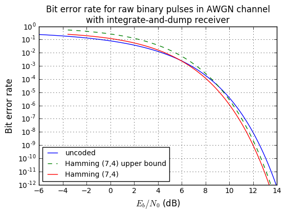

Both the exact calculation and the upper bound are fairly close.

We can do something similar with Reed-Solomon error rates. For an $ (n,k) = (255,255-2t) $ Reed-Solomon code, with transmitted bit error probability $ p $, the error probability per byte is $ q = 1 - (1-p)^8 $, and there are a couple of situations, given the number of byte errors $ v $ per 255-byte block:

$ v \le t $: Reed-Solomon will decode them all correctly, and the number of decoded byte errors is zero.
$ v > t $: More than $ t $ byte errors: This is the tricky part.
- Best-case estimate: we are lucky and the decoder actually corrects $ t $ errors, leading to $ v-t $ errors. This is ludicrously optimistic, but it does represent a lower bound on the bit error rate.
- Worst-case estimate: we are unlucky and the decoder alters $ t $ values which were correct, leading to $ v+t $ errors. This is ludicrously pessimistic, but it does represent an upper bound on the bit error rate.
- Empirical estimate: we can actually generate some random samples covering various numbers of errors, and see what a decoder actually does, then use the results to extrapolate a data bit error rate. This will be closer to the expected results, but it can take quite a bit of computation to generate enough random samples and run the decoder algorithm.

OK, now we’re going to tie all this together and show four graphs:

Bit error rate of the decoded data (after error correction) vs. raw bit error rate during transmission. This tells us how much the error rate decreases.
- One graph will show large scale error rates.
- Another will show the same data in closer detail.
Bit error rate of the decoded data vs. $ E_b/N_0 $. This lets us compare bit error rates by how much transmit energy they require to achieve that error rate.
Effective gain in $ E_b/N_0 $, in decibels, vs. bit error rate of the decoded data.

# Codes under analysis:
class RawAnalyzer(object):
    def bit_error_rate(self, p):
        return p
    @property
    def codename(self):
        return 'uncoded'
    @property
    def rate(self):
        return 1

ha74 = HammingAnalyzer(0b1011)
ha1511 = HammingAnalyzer(0b10011)
analyzers = [RawAnalyzer(), ha74, ha1511,
            ReedSolomonWorstCaseAnalyzer(255,253),
            ReedSolomonBestCaseAnalyzer(255,253),
            ReedSolomonMonteCarloAnalyzer(
              rs.RSCoder(255,253,generator=2,prim=0x11d,fcr=0,c_exp=8))
                 .set_simulation_sample_counts([10]
                    +[10000,5000,2000,1000,1000,1000,1000,1000]
                    +[100]*10),
            ReedSolomonWorstCaseAnalyzer(255,251),
            ReedSolomonBestCaseAnalyzer(255,251),
            ReedSolomonMonteCarloAnalyzer(
              rs.RSCoder(255,251,generator=2,prim=0x11d,fcr=0,c_exp=8))
                 .set_simulation_sample_counts([10]
                    +[10000,5000,2000,1000,1000,1000,1000,1000]
                    +[100]*5),
            ReedSolomonWorstCaseAnalyzer(255,247),
            ReedSolomonBestCaseAnalyzer(255,247),
            ReedSolomonMonteCarloAnalyzer(
              rs.RSCoder(255,247,generator=2,prim=0x11d,fcr=0,c_exp=8))
                 .set_simulation_sample_counts([10]
                    +[10000,5000,2000,1000,1000,1000,1000,1000]
                    +[100]*5),
            ReedSolomonWorstCaseAnalyzer(255,239),
            ReedSolomonBestCaseAnalyzer(255,239),
            ReedSolomonMonteCarloAnalyzer(
              rs.RSCoder(255,239,generator=2,prim=0x11d,fcr=0,c_exp=8))
                 .set_simulation_sample_counts([10]
                    +[10000,5000,2000,1000,1000,1000,1000,1000]),
            ReedSolomonWorstCaseAnalyzer(255,223),
            ReedSolomonBestCaseAnalyzer(255,223),
            ReedSolomonMonteCarloAnalyzer(
              rs.RSCoder(255,223,generator=2,prim=0x11d,fcr=0,c_exp=8))
                 .set_simulation_sample_counts([10]
                    +[5000,2000,1000,500,500,500,500,500]),
            ReedSolomonWorstCaseAnalyzer(255,191),
            ReedSolomonBestCaseAnalyzer(255,191),
            ReedSolomonMonteCarloAnalyzer(
              rs.RSCoder(255,191,generator=2,prim=0x11d,fcr=0,c_exp=8))
                 .set_simulation_sample_counts([10]
                    +[2000,1000,500,500,500,500,500,500]),
            ]
styles = ['k','r','g','b--','b--','b','c--','c--','c',
          'm--','m--','m',
          '#88ff00--','#88ff00--','#88ff00',
          '#ff8800--','#ff8800--','#ff8800',
          '#888888--','#888888--','#888888']

# Sigh. This takes a while.
import time

for analyzer in analyzers:
    if hasattr(analyzer, 'simulate'):
        print "RS(%d,%d)" % (analyzer.n, analyzer.k)
        np.random.seed(123)  
        # just to make the Monte Carlo analysis repeatable
        t0 = time.time()
        analyzer.simulate()
        t1 = time.time()
        print "%.2f seconds" % (t1-t0)

RS(255,253)
42.47 seconds
RS(255,251)
44.90 seconds
RS(255,247)
62.66 seconds
RS(255,239)
151.81 seconds
RS(255,223)
197.57 seconds
RS(255,191)
470.05 seconds

ebno_db = np.arange(-6,18,0.02)
ebno = 10**(ebno_db/10)
# Decibels are often confusing.
# dB = 10 log10 x  if x is measured in energy
# dB = 20 log10 x  if x is measured in amplitude. 

# Raw bit error probability
p = Q(np.sqrt(2*ebno))
# Binomial distribution -- this is used by the RS Monte Carlo analyzers
pbinom = scipy.stats.binom.pmf(np.atleast_2d(np.arange(800)).T,255*8,p)

error_rates = [analyzer.bit_error_rate(p) for analyzer in analyzers]

colors = [s[:-2] if s.endswith('--') else s for s in styles]
linestyles = ['--' if s.endswith('--') else '-' for s in styles]
def label_for(analyzer):
    codename = analyzer.codename
    if codename.endswith(' worstcase'):
        return None
    elif codename.endswith(' bestcase'):
        return codename[:-8] + 'bounds'
    else:
        return codename

# 1a and 1b. Raw vs. derived probability

for xscale,yscale in [(1e-12,1e-20),(1e-5,1e-8)]:
    fig = plt.figure(figsize=(7,6))
    ax = fig.add_subplot(1,1,1)
    for i, analyzer in enumerate(analyzers):
        p2 = error_rates[i]
        ax.loglog(p, p2, 
                  color=colors[i], linestyle=linestyles[i], label=label_for(analyzer))
    ax.set_xlabel('Raw bit error rate')
    ax.set_ylabel('Data bit error rate')
    ax.legend(loc='upper left',fontsize=8, labelspacing=0, handlelength=3)
    ax.grid('on')
    ax.set_title('Code effect on data bit error rate')
    ax.set_xlim(xscale,0.5)
    ax.set_ylim(yscale,1)

# 2. Data error rate vs. Eb/N0
fig = plt.figure(figsize=(7,6))
ax = fig.add_subplot(1,1,1)
for i, analyzer in enumerate(analyzers):
    p2 = error_rates[i]
    
    ax.semilogy(dBE(ebno/analyzer.rate), p2, 
                color=colors[i], linestyle=linestyles[i], label=label_for(analyzer))
ax.set_ylabel('Data bit error rate',fontsize=12)
ax.set_xlabel('$E_b/N_0$ (dB)',fontsize=12)
ax.set_xlim(-6,14)
ax.set_xticks(np.arange(-6,15,2))
ax.set_ylim(1e-12,1)
ax.legend(loc='lower left',fontsize=8, labelspacing=0, handlelength=3)
ax.grid('on')
ax.set_title('Data bit error rate for raw binary pulses in AWGN channel\n'
          +'with integrate-and-dump receiver');

# 3. Eb/No gain vs. data error rate
fig = plt.figure(figsize=(7,6))
ax = fig.add_subplot(1,1,1)
for i, analyzer in enumerate(analyzers):
    p2 = error_rates[i]
    ebno_equiv = Qinv(p2)**2/2
    ax.semilogx(p2, dBE(ebno_equiv*analyzer.rate/ebno),
                    color=colors[i], linestyle=linestyles[i], label=label_for(analyzer))
ax.set_xlim(1e-16,0.5)
ax.set_ylim(-8,10)
ax.set_yticks(np.arange(-8,10.1,2))
ax.legend(loc='lower left',fontsize=8, labelspacing=0, handlelength=3)
ax.set_xlabel('Data bit error rate', fontsize=12)
ax.set_ylabel('Gain (dB)', fontsize=12)
ax.grid('on')
ax.set_title('Effective $E_b/N_0$ gain vs data bit error rate');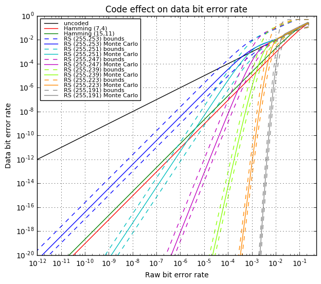

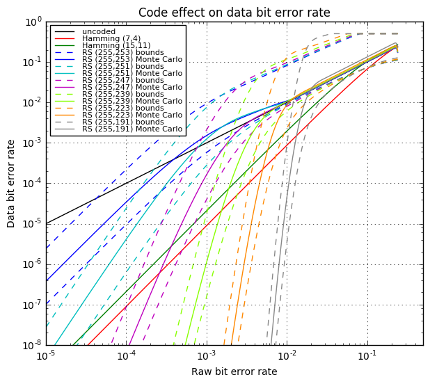
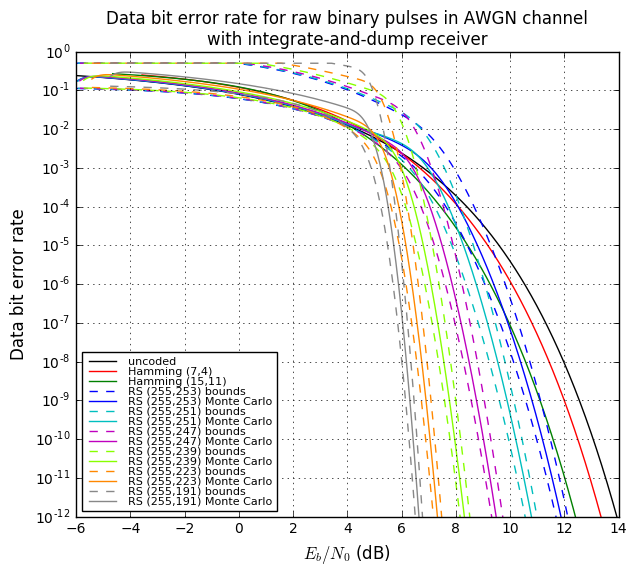
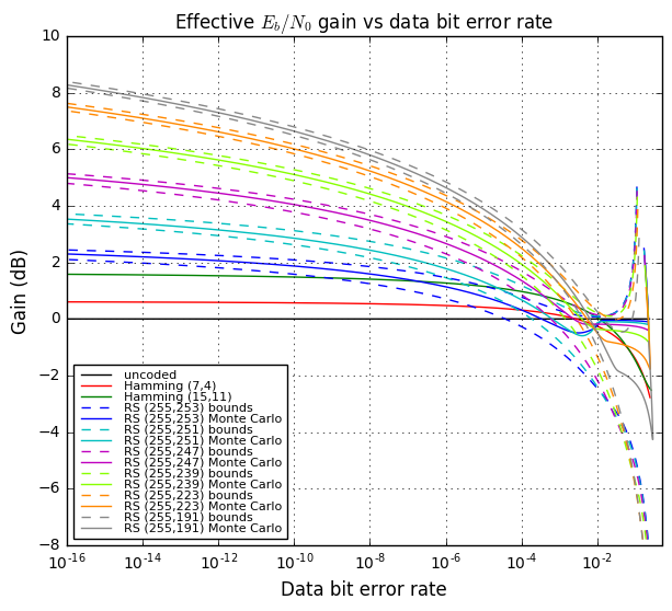
OK, so what are we looking at here?

The top two graphs show us a few things:

At low channel bit error rates (= “raw bit error rate”), the effective data bit error rate can be made much lower. For example, at a $ 10^{-4} $ channel bit error rate, a Hamming (7,4) code can bring the effective data bit error rate down to about $ 10^{-7} $, and an RS(255,239) code can bring the effective data bit error rate down to about $ 10^{-14} $. Much lower, and we don’t have to sacrifice much bandwidth to do it; the code rate of RS(255,239) is 239/255 ≈ 0.9373.
At high channel bit error rates, on the other hand, the effective data bit error rate may not be much better, and may even be a little higher than the channel data bit error rate. It looks like on average this could be about a factor of 2 worse, in the cases of low-robustness Reed-Solomon codes like RS(255,253) and RS(255,251).
The meaning of “low” and “high” channel bit error rates depends on the coding technique used. Hamming codes are short, so you still see benefits from them at channel bit error rates as high as 0.2, whereas RS(255,251) doesn’t help decrease the error rate unless you have channel bit error rates below 0.0005, and the higher-robustness Reed-Solomon codes like RS(255,223) and RS(255,191) work well up to error rates of about 0.01.

The bottom two graphs show us how this reduction in effective bit error rate trades off against the $ E_b/N_0 $ penalty we get for using up part of our channel capacity for the redundancy of parity bits. (Remember, longer average transmission times per bit times mean that we need a larger $ E_b $ per encoded data bit.)

Hamming codes can gain between 0.5-1.5dB of $ E_b/N_0 $ compared to uncoded data, for the same effective data bit error rate.
Reed-Solomon codes can gain between 2-10dB of $ E_b/N_0 $ compare to uncoded data, for the same effective data bit error rate.
This gain works better at low channel bit error rates; the advantages in $ E_b/N_0 $ compared to uncoded data show up if the data bit error rate is somewhere below the 0.0001 to 0.01 range. Reed-Solomon codes beat Hamming codes once you get below about 0.005 data bit error rate, at least for the high-robustness codes; the Reed-Solomon codes which don’t add much redundancy, like RS(255,253), don’t beat Hamming codes unless the data bit error rate is below $ 10^{-7} $.
At high effective bit error rates, the coded messages can have worse performance in terms of $ E_b/N_0 $ for the same effective data bit error rate.
We generally want low effective bit error rates anyway; something in the $ 10^{-6} $ to $ 10^{-12} $ range is probably reasonable, depending on the application and how it is affected by errors. Those applications that have other higher-level layers which can handle retries in case of detected errors, can usually get away with bit error rates of $ 10^{-6} $ or even higher. Storage applications, on the other hand, need to keep errors low, because there’s no possible mechanism for retransmission; the only way to deal with it is to add another layer of error correction — which is something that is used in certain applications.

Why Not Use Reed-Solomon Instead of a CRC?

So here’s a question that might come to mind. Consider the following two pairs of cases:

RS(255,253) vs. a 253-byte packet followed by a 16-bit CRC
RS(255,251) vs. a 251-byte packet followed by a 32-bit CRC

Within each pair, there is the same overhead, and about the same encoding complexity and memory requirements if a lookup-table-based encoder is used. Decoders that check for the presence of transmission errors are essentially the same complexity as an encoder; it’s only the error-correction step that takes more CPU horsepower.

A CRC can be used to detect errors, but not to correct them. A Reed-Solomon code can be used to detect errors, up to 1 byte error in case of RS(255,253) and two byte errors in case of RS(255,251).

So why shouldn’t we be using Reed-Solomon instead of a CRC?

Well, CRCs are meant for detecting a small number of bit errors with guaranteed certainty. Reed-Solomon codes are designed to handle byte errors, and that means bursts of a byte or two, depending on the code parameters. So the nature of the received noise may make a big difference in terms of which is better. Noise models like AWGN, where the likelihood of any individual bit error is independent of any other, favor bit-error detection techniques; noise models in which multi-bit bursts are common will favor Reed-Solomon.

But the biggest impact is that by allowing error correction, we give up some of our ability to detect errors. I mentioned this toward the end of Part XV. Let’s look at it again.

Dry Imp Net Nrp Nmy

Let’s take a look at our fictitious dry imp net encoding scheme again. Three codewords — dry, imp, and net — and three symbols per word.

This encoding scheme has a Hamming distance of 3, which means we can detect up to 2 errors or correct up to 1 error.

If we don’t do any error correction, there are only 3 codewords out of 27 possible messages, so our ability to detect invalid messages is very good. The only way we’re going to misinterpret dry as imp or net is if we happen to get the right kind of error to switch from one valid codeword to another, which needs three simultaneous errors.

On the other hand, if we do decide to use error correction, then all of a sudden we have 21 acceptable messages. By “acceptable” I mean a message that is either correct or correctable. If we get a message like dmp that was originally dry, sorry, we’re going to turn it into imp, because that’s the closest codeword. The only unacceptable messages are nrp, nmy, iey, irt, dmt, and dep, which have a minimum distance of 2 to any codeword.

There are a few limited codes — Hamming codes are one of them — which have the property that there are no unacceptable messages. These are called perfect codes, and it means that any received message is either correct or can be corrected to the closest codeword. Here we have to assume that errors are infrequent, and if we do get more errors than we can correct, then we are just going to make an erroneous correction. Oh well.

I looked into this a little bit for Reed-Solomon codes. For $ RS(255,255-2t) $, it looks like $ t=1 $ is close to perfect, and $ t=2 $ isn’t too far away either, but as you start adding more redundancy symbols, the number of uncorrectable messages increases much faster than the number of correctable messages, and these boundaries around each codeword — which are called Hamming spheres, even though they’re more like N-dimensional hypercubes — cover less and less of the message space. Which is good, at least for error detection, because it means we’re more likely to be able to detect errors even if there are more than $ t $ of them.

Below is some data from the Monte Carlo simulations I used to compute bit error rates — this time presented a little differently, showing tables of what happens when there are more than $ t $ errors. Each random error pattern of $ v $ bit errors (and note that this may produce less than $ v $ byte errors, if more than one error occurs in the same byte) can have three outcomes:

CORRECT: the error pattern decodes correctly
FAIL: the decoding step fails, so we don’t change the received message, and the number of received errors stays the same
WORSEN: the error pattern decodes incorrectly, to a different codeword

The table shows the number of samples nsample in each case, and the fraction of those samples that fall into the CORRECT, FAIL, and WORSEN outcomes.

rsanalyzers = [analyzer for analyzer in analyzers
               if isinstance(analyzer, ReedSolomonMonteCarloAnalyzer)]
def summarize_simulation_results(sr):
    shist, fhist = sr
    nfail = sum(fhist)
    nsample = nfail + sum(shist)
    ncorrect = shist[0]
    nworsen = sum(shist[1:])
    return (nsample,
            ncorrect*1.0/nsample, 
            nfail*1.0/nsample,
            nworsen*1.0/nsample)
data = [(analyzer.n, analyzer.k, analyzer.t, i+analyzer.t)
       +summarize_simulation_results(sr)
    for analyzer in rsanalyzers
    for i, sr in enumerate(analyzer.simulation_results)
    if i > 0 and i <= 8]
df = pd.DataFrame(data,
            columns='n k t v nsample ncorrect nfail nworsen'.split())
df.set_index(['n','k','t','v'])

				nsample	ncorrect	nfail	nworsen
n	k	t	v
255	253	1	2	10000	0.0029	0.1228	0.8743
			3	5000	0.0000	0.0000	1.0000
			4	2000	0.0000	0.0490	0.9510
			5	1000	0.0000	0.0000	1.0000
			6	1000	0.0000	0.0130	0.9870
			7	1000	0.0000	0.0000	1.0000
			8	1000	0.0000	0.0140	0.9860
			9	1000	0.0000	0.0000	1.0000
	251	2	3	10000	0.0091	0.4998	0.4911
			4	5000	0.0000	0.5036	0.4964
			5	2000	0.0000	0.5115	0.4885
			6	1000	0.0000	0.4850	0.5150
			7	1000	0.0000	0.5110	0.4890
			8	1000	0.0000	0.4940	0.5060
			9	1000	0.0000	0.5190	0.4810
			10	1000	0.0000	0.5070	0.4930
	247	4	5	10000	0.0342	0.9288	0.0370
			6	5000	0.0004	0.9628	0.0368
			7	2000	0.0000	0.9490	0.0510
			8	1000	0.0000	0.9650	0.0350
			9	1000	0.0000	0.9710	0.0290
			10	1000	0.0000	0.9650	0.0350
			11	1000	0.0000	0.9710	0.0290
			12	1000	0.0000	0.9610	0.0390
	239	8	9	10000	0.1213	0.8787	0.0000
			10	5000	0.0102	0.9898	0.0000
			11	2000	0.0000	1.0000	0.0000
			12	1000	0.0000	1.0000	0.0000
			13	1000	0.0000	1.0000	0.0000
			14	1000	0.0000	1.0000	0.0000
			15	1000	0.0000	1.0000	0.0000
			16	1000	0.0000	1.0000	0.0000
	223	16	17	5000	0.3796	0.6204	0.0000
			18	2000	0.0930	0.9070	0.0000
			19	1000	0.0200	0.9800	0.0000
			20	500	0.0020	0.9980	0.0000
			21	500	0.0000	1.0000	0.0000
			22	500	0.0000	1.0000	0.0000
			23	500	0.0000	1.0000	0.0000
			24	500	0.0000	1.0000	0.0000
	191	32	33	2000	0.8490	0.1510	0.0000
			34	1000	0.5580	0.4420	0.0000
			35	500	0.3160	0.6840	0.0000
			36	500	0.1700	0.8300	0.0000
			37	500	0.0720	0.9280	0.0000
			38	500	0.0220	0.9780	0.0000
			39	500	0.0080	0.9920	0.0000
			40	500	0.0020	0.9980	0.0000

The interesting trends here are

For RS(255,253), with more than 1 error, the outcome is usually WORSEN. With $ v=2 $ errors we occasionally get a successful correction. Compared to a 16-bit CRC, we risk making errors worse by trying to correct them, so unless we have a system with very low probability of 2 or more errors, we are better off using a 16-bit CRC and not trying to correct errors.
For RS(255,251), with more than 2 errors, the outcome is about a 50-50 split between FAIL and WORSEN. With $ v=3 $ errors we occasionally get a successful correction. Compared to a 32-bit CRC, we risk making errors worse by trying to correct them. It’s not as bad as RS(255,253), but a 50% chance of making things worse if there are three or more errors, makes it more attractive to use a 32-bit CRC.
For RS(255,247), with more than 4 errors, the outcome is usually FAIL with a small probability of WORSEN. With $ v=4 $ and $ v=5 $ errors we occasionally get a successful correction. Compared to a 64-bit CRC, now the use of Reed-Solomon becomes much more attractive, at least for packets of length 255 or less.
For RS(255,239) and other decoders with higher $ t $ values, the output almost never is WORSEN. Probability of CORRECT becomes greater even though we are beyond the Hamming bound of at most $ t $ correctible errors. Reed-Solomon is very attractive, but the encoding cost starts to get higher.

These probabilities of a WORSEN outcome are fairly close to their theoretical values, which are just the fraction of all possible messages which are within a Hamming distance of $ t $ of a valid codeword.

For example, if we have RS(255,253), then the last two bytes of valid codewords are completely dependent on the preceding bytes, so the fraction of valid codewords is $ 1/256^2 = 1/65536 $, and the fraction of all possible messages which are within a distance of 1 of those valid codewords is $ \frac{1 + 255 \times 255}{256^2} \approx 0.9922 $. For each codeword we have one message with distance 0 (the codeword itself) and $ 255 \times 255 $ messages with distance 1: each of the 255 message bytes can be corrupted with 255 other values.

Or if we have RS(255,251), this fraction becomes $ \frac{1 + 255 \times 255 + \frac{255 \times 254}{2} \times 255^2}{256^4} \approx 0.4903 $.

The general formula for this fraction is

$$\rho(t) = 256^{-2t}\sum\limits_{j=0}^t {255\choose j}255^j$$

which we can graph:

def rscoverage(t):
    y = 0
    p = 1.0/256
    x = 1.0
    for k in xrange(t+1):
        u = x
        for j in xrange(2*t-k):
            if j < k:
                u *= 255.0/256
            else:
                u *= p
        y += u
        x *= (255-k)/256.0
        x /= k+1
    return y

tlist = np.arange(1,21)
fig=plt.figure()
ax=fig.add_subplot(1,1,1)
ax.semilogy(tlist,[rscoverage(t) for t in tlist],'.')
ax.set_title('Fraction of messages in $RS(255,255-2t)$\n within distance $t$ of a valid codeword')
ax.set_xlabel('$t$',fontsize=12)
ax.set_ylabel('$\\rho$',fontsize=12)
ax.grid('on')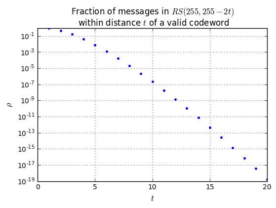

The sweet spot for low-end embedded systems is probably to use Reed-Solomon (255,247), where $ t=4 $. Possibly (255,239), where $ t=8 $. Smaller values of $ t $ allow a table-based implementation with a minimum amount of CPU time and memory; larger values of $ t $ lower the probability of erroneous correction.

But the most important thing is really to understand the behavior of errors in your system:

Probability of errors – run some tests and try to figure out the rate of errors without any attempt at error correction. A system with an average error rate of 1 error per $ 10^{6} $ bytes is a much different system to work with, than one that has an average error rate of 1 error per 1000 bytes.
Impact of errors – if you’re working with audio data, an error might sound like a brief “pop” in the sound, and this may not be a big deal. If you have a sensor gathering and transmitting data from a once-in-a-lifetime experiment, and losing data can make or break the results, then error correction coding is relatively cheap insurance.

Real-world Applications of Reed-Solomon Codes

Reed-Solomon codes are now in widespread use.

We already talked about the use of Reed-Solomon codes in the Voyager space probes from Uranus and Neptune onwards. They have been supplanted in more recent NASA missions, such as the Mars Reconaissance Encoder by turbo codes, which have higher $ E_b/N_0 $ gain.

Compact discs and DVDs use cross-interleaved Reed-Solomon encoding to increase the robustness against errors even if they show up as scratches impacting large numbers of bits.

Broadband data transmission systems like VDSL2 use Reed-Solomon codes to reduce error rates for a given transmitter energy.

The application I find most interesting is in QR codes, where Reed-Solomon codes are used along with a clever scheme to distribute the data bits spatially over a wide area. This makes them robust to severe data loss errors.

Normally you see QR code images like this:

But they can still be decoded even when part of the information has been corrupted, like this:

or this:

or even this:

I couldn’t find a QR code application that outputs the raw binary bits before decoding, but it would be interesting to see how many errors or erasures these images have. The four levels of error correction in a QR code, L, M, Q, and H, allow up to 30% errors by requiring more bits to encode a given message. The code above is an H-level code, and I kept adding larger and larger disturbances until the decoder was unable to process an image; these are slightly below the failure point, so they are probably in the 25-30% range.

Wrapup

OK! We’ve wandered around the topic of Reed-Solomon codes today, covering a few important points:

Reed-Solomon codes represent messages as polynomials with coefficients in $ GF(2^m) $, and are often denoted as $ RS(n,k) $
The Reed-Solomon $ (255,255-2t) $ code is a common subset, representing a codeword as 255 bytes, each byte an element of $ GF(2^8) $. This allows for correction of up to $ t $ errors or $ 2t $ erasures.
To specify a particular Reed-Solomon code, in addition to knowing $ n $ and $ k $, you need the characteristic polynomial of the symbol field — for $ GF(2^8) $, this is a degree 8 polynomial — and the generator polynomial, which is of the form $ g(x) = (x+\lambda^b)(x+\lambda^{b+1})(x+\lambda^{b+2})\ldots (x+\lambda^{b+2t-1}) $, where $ b $ is an integer and $ \lambda $ is any generating element in $ GF(2^8) $ — meaning that all nonzero elements of $ GF(2^8) $ are expressible as $ \lambda^i $ for some integer $ i $ between 0 and 254. The important property of $ g(x) $ is that its roots are $ 2t $ consecutive powers of $ \lambda $.
Algebraically, encoding a message involves expressing it as a polynomial $ M(x) $, computing $ r(x) = x^{2t}M(x) \bmod g(x) $ and constructing the codeword $ C_t(x) = x^{2t}M(x) + r(x) $
In practical terms, we can encode a message using an LFSR where the shift cells contain elements of $ GF(2^8) $ and the LFSR taps are multiplier coefficients in $ GF(2^8) $, each tap corresponding to the corresponding coefficient in the generator polynomial.
This LFSR approach can be implemented using lookup tables to handle the finite field mathematics
Decoding takes considerably more processing power, and we didn’t cover the details in this article.
Shortened Reed-Solomon codes are used by taking an $ (n,k) $ code and using it as an $ (n-l,k-l) $ code, where both transmitter and receiver assume that there are $ l $ implicit zeros at the beginning of the message.
Calculating bit error rates is a pain. But if you do it right, you will end up with curves of data bit error rate vs. $ E_b/N_0 $, like this graph:

Higher values of $ t $ reduce the code rate somewhat, but allow for greater gains in $ E_b/N_0 $ for the same data bit error rate. (Or alternatively, much lower data bit error rates for the same amount of signal energy per bit per unit noise.)
Use of error correction reduces the robustness to error detection, especially at low values of $ t $, but for $ t > 4 $ or so, the probability of mistakenly correcting more than $ t $ errors to the wrong codeword is very small. The vast majority of the time if there are more than $ t $ errors, the decoder just fails and the number of errors remains unchanged. There are cases with more than $ t $ errors where the decoder would produce a correction to the wrong codeword, but it has a low probability unless the errors are introduced intentionally.
Reed-Solomon has lots of applications for reducing the probability of errors: space transmission, storage formats like CDs and DVDs, QR codes, and DSL.

That’s all for today!

Next time we will tackle an interesting problem relating to CRCs.

References

Error-Correcting Codes:

Gregory Mitchell, ARL-TR-4901: Investigation of Hamming, Reed-Solomon, and Turbo Forward Error Correcting Codes, US Army Research Laboratory, July 2009.

Reed-Solomon / BCH codes:

C.K.P. Clarke, WHP031: Reed-Solomon Error Correction, British Broadcasting Corporation, January 2002.
William Geisel, NASA Technical Memorandum 102162: Tutorial on Reed-Solomon Error Correction Coding, National Aeronautics and Space Administration, August 1990.
John Gill, EE 387 Notes 7: BCH and Reed-Solomon Codes, Stanford University, 2014.
Fabrizio Pollara, A Software Simulation Study of a (255,223) Reed-Solomon Encoder-decoder, Jet Propulsion Laboratory, JPL Publication 85-23, April 1985. (This report is interesting because it contains C code for both an encoder and decoder. I have not tried to use either, and it’s nearly unreadable code, using short cryptic identifiers everywhere.)
Duke University, CPS296 and notes on decoding.
Wikiversity, Reed-Solomon Codes for Coders
I. S. Reed and G. Solomon, Polynomial Codes over Certain Finite Fields, Journal of the Society for Industrial and Applied Mathematics, Volume 8, issue 2, pp. 300–304, June 1960.
Yasuo Sugiyama, Masao Kasahara, Shigeichi Hirasawa, and Toshihiko Namekawa, A Method for Solving Key Equation for Decoding Goppa Codes, Information and Control Volume 27, issue 1, January 1975, pp 87-99.

AWGN Channels:

Dilip Sarwate, ECE 361: Lecture 3: Matched Filters – Part I, 2011. This has the equation for determining the variance of received white noise after it goes through a filter $ h(t) $.

QR Codes:

Bill Casselman, How to Read QR Symbols Without Your Mobile Telephone, American Mathematical Society, 2013.

You might also like... (promoted content)

Check out Memfault's New Sandbox!

Upcoming Course - Python Applications for Digital Design and Signal Processing

The 2024 Embedded Online Conference - Register Early and Save with Promo Code ER2024!

Comments

Comments
Write a Comment

Select to add a comment

To post reply to a comment, click on the 'reply' button attached to each comment. To post a new comment (not a reply to a comment) check out the 'Write a Comment' tab at the top of the comments.

Please login (on the right) if you already have an account on this platform.

Otherwise, please use this form to register (free) an join one of the largest online community for Electrical/Embedded/DSP/FPGA/ML engineers:

Choose a Username

E-Mail (Work, School or ieee)

First Name

Last Name

Employer

Job Title

Country

State

Password

Confirm Password

By checking this box, I agree with the terms of use and privacy policy By checking this box, I consent to receive occasional emails from the *Related sites and their partners. I understand that these emails will only contain relevant information and that I can unsubscribe at any time.

Linear Feedback Shift Registers for the Uninitiated, Part XVI: Reed-Solomon Error Correction

Reed-Solomon Codes

Details of Reed-Solomon Encoding

Reed-Solomon in Python

Mama’s Little Baby Loves Shortnin’, Shortnin’, Mama’s Little Baby Loves Shortnin’ Bread

Why does it work?

Reed-Solomon Encoding in `libgf2`

Chocolate Strawberry Peach Vanilla Banana Pistachio Peppermint Lemon Orange Butterscotch

C Implementation

Is It Worth It?

Bit Error Rate Calculations Are the Bane of My Existence

Why Not Use Reed-Solomon Instead of a CRC?

Dry Imp Net Nrp Nmy

Real-world Applications of Reed-Solomon Codes

Wrapup

References

Sign in

You might also like...

About Jason Sachs

Popular Posts by Jason Sachs

Blogs - Hall of Fame

Free PDF Downloads

Quick Links

About EmbeddedRelated.com

Social Networks

The Related Media Group

Linear Feedback Shift Registers for the Uninitiated, Part XVI: Reed-Solomon Error Correction

Reed-Solomon Codes

Details of Reed-Solomon Encoding

Reed-Solomon in Python

Mama’s Little Baby Loves Shortnin’, Shortnin’, Mama’s Little Baby Loves Shortnin’ Bread

Why does it work?

Reed-Solomon Encoding in libgf2

Chocolate Strawberry Peach Vanilla Banana Pistachio Peppermint Lemon Orange Butterscotch

C Implementation

Is It Worth It?

Bit Error Rate Calculations Are the Bane of My Existence

Why Not Use Reed-Solomon Instead of a CRC?

Dry Imp Net Nrp Nmy

Real-world Applications of Reed-Solomon Codes

Wrapup

References

Sign in

You might also like...

About Jason Sachs

Popular Posts by Jason Sachs

Blogs - Hall of Fame

Free PDF Downloads

Quick Links

About EmbeddedRelated.com

Social Networks

The Related Media Group

Reed-Solomon Encoding in `libgf2`