


March is Oscilloscope Month — and at Tim Scale!
I got my oscilloscope today.
Maybe that was a bit of an understatement; I'll have to resort to gratuitous typography:
I GOT MY OSCILLOSCOPE TODAY!!!!
Those of you who are reading this blog may remember I made a post about two years ago about searching for the right oscilloscope for me. Since then, I changed jobs and have been getting situated in the world of applications engineering, working on motor control projects. I've been gradually working to fill in gaps in the infrastructure available to me and my coworkers, and one of those has been an oscilloscope I can use in my office. Our group's budget recently allowed us to fill in some of those gaps. So:
I got my oscilloscope today! And it's even the one I asked for!
No, wait — it's better than the one I asked for! Here's why:
The oscilloscope I asked for was an MSOX3024A. When I got a quote from a distributor, they said there was a promotion from Agilent, and they could offer me a lower price. Agilent has a deal ("Supercharge Your Bandwidth!") that runs until March 31. Most oscilloscope models come in series, with different bandwidth options. You want a less expensive scope? Pick the lowest bandwidth. You want something with a high bandwidth? It'll cost you. So the Agilent deal offers you the scope you want at the price of the next lower bandwidth. I would get a MSOX3024A (200MHz) at the normal price of an MSOX3014A (100MHz). Net savings: about $350. Yay! Quote obtained, forwarded on to manager, no problem, back to work.
And then I got this funny nagging hunch in the back of my mind. MSOX3024A at the normal price of the MSOX3014A... hmmm... hmmm... what about the MSOX3034A at the normal price of the MSOX3024A? I checked Agilent's list prices for the MSOX3000 series:
| MSOX3014A | 100MHz | $5199 |
| MSOX3024A | 200MHz | $5556 |
| MSOX3034A | 350MHz | $9169 |
| MSOX3054A | 500MHz | $11993 |
| MSOX3104A | 1GHz | $15819 |
Goodness, I could save $3500! I called the distributor back and asked if the promotion applied to the MSOX3034A. Yep. Some quick discussions and pleading with my manager and we got the order in for the MSOX3034A. Woot!
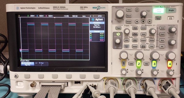
So I got my oscilloscope today. (Did I mention that yet?) First action of the day: put the probes on the scope along with the little color coded bands to help you keep the channels from getting mixed up, and compensate the scope probes.
What? You've never compensated an oscilloscope probe before? It's easy. You connect the probe to the calibration signal post on the front panel. It's a precision square wave. Then you zoom up the vertical scale so you can see the transients. Here's the deal: The scope comes with BNC connectors, and most scopes these days allow you to configure the input impedance with one of two choices. If you are doing high frequency measurements, they're typically 50Ω characteristic impedance to avoid reflections. If you are doing lower frequency measurements on high-impedance nodes of a circuit, you don't want the oscilloscope loading down the input, so you pick the other option, which is usually 1MΩ input impedance. But that's not good enough for most applications, and usually you want a probe with a voltage divider so you can get the input impedance higher, and have a higher acceptable input voltage range. Typical scope probes are 10x probes, which mean they have a 10:1 voltage divider inside, and are therefore 10MΩ input impedance.
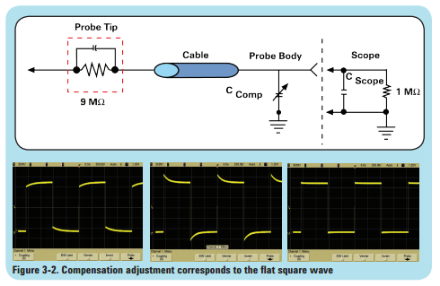
(Figure from Agilent's Application Note 1603: Eight Hints for Better Scope Probing )
Now, both the probe tip and the oscilloscope itself have parasitic input capacitance. If these aren't matched with the resistor divider, the probe will give you a transfer function that is frequency-dependent, and the waveforms you see on the scope will be distorted. So oscilloscope probe manufacturers usually put a variable capacitor in the probe, either near the probe tip or near the BNC end of the probe, so they can match the input network and make it close to frequency independent. If you connect the probe to a square wave, you can tune the variable capacitor so that the square wave has edges that are square, and not rounded off or with an overshoot. The variable capacitor has a slotted adjustment screw, and usually you want to use a nonconducting nonferrous screwdriver to prevent the signal from being altered while you're turning the screw. Scopes usually come with a little plastic mini-screwdriver you can use to adjust the capacitor screw.
Waveform data transfer
I talked a little bit about waveform data transfer in my 2012 article. Gone are the days of DB9 RS232 connections (get out your null modems and gender changers!) and floppy disk drives. Now everything's either thumb drive or USB or Ethernet. The MSOX3000 series offers all three, but only the USB host (for thumb drive) and USB device connectors are built-in to the oscilloscope; Ethernet connector ("LAN port") costs extra.
But at least the basic software is free. Agilent offers free I/O libraries which include device drivers for USB and Virtual Instrument Software Architecture (VISA) libraries.
As far as application software: yeah, you can buy some software from Agilent, but I learned long ago that most software from oscilloscope manufacturers isn't very good. (WaveStar ring a bell for anyone out there with a Tektronix scope?) And I'm a big fan of Python, if you haven't figured that out already from previous columns. So of course I looked around for a Python program to download the Agilent waveforms.
I quickly found an IPython notebook on interfacing to Agilent oscilloscopes using their VISA libraries and the pyvisa Python library. Cool!
It took me a while to get things running, but I was able to connect to my oscilloscope via USB and interact with it in IPython. A couple of stumbling blocks:
- pyvisa requires a .pyvisarc file to point to the visa32.dll file you install with Agilent's IO. The pyvisa version 1.4 needs you to do this manually. Version 1.5 (still in development) is supposed to locate this file automatically.
-
pyvisa is a low-level library which only facilitates the communication with a scope. You still have to use the required ASCII command/response protocol given in Agilent's programming guide, which looks like this:
scope = instrument("TCPIP0::130.30.240.155::inst0::INSTR")
# Connect to the scope using the VISA address (see below)
scope.ask("*IDN?") # Query the IDN properties of the scope
sa_rate = float(scope.ask(":ACQ:SRAT:ANAL?"))
# Get the scope's sample rate
This just screams for someone to write a higher-level library to interface with these series of oscilloscopes. I'll probably end up writing one that is mediocre and not something I can share outside my company. It's really something that Agilent should provide: they don't seem to realize that there is a whole scientific community out there which likes using Python rather than Visual Basic or C#.
In any case, I haven't finished downloading waveforms yet, but one cool thing is that you can set the time scale of the oscilloscope with the :TIMe:SCALE command:
scope.write(":TIM:SCALE 10e-6")
Shazaam! Your scope is now set to 10 μs/division. But that's not all! Let's say you want exactly 3.21 μs/division. You can do that with these scopes, but it's a pain to do, you need to fiddle with the coarse and fine time adjustment knobs. Or:
scope.write(":TIM:SCALE 3.21e-6")
Pow! It just works!
Anyway, that's what I've been up to so far. If I run into something else cool, I'll share it in a future article.
Thanks to Microlease for giving us a good price on these scopes. If you're buying stuff from Agilent, give them a holler — don't just settle for the Agilent list prices.
Update on Mar 6:
I stand corrected: Agilent does include some sample Python code to interface with the MSOX3000 oscilloscopes. It's on p. 1221 of the Programming Guide, and uses pyvisa — well, an earlier version of it, at least. (By the way, those weird :TIM:SCALE commands are called SCPI)
But it's not very "pythonic"; it looks like a Visual Basic programmer was told "You! Translate this into Python! We need Python sample code!" There are global variables and redundant function calls and then there's a sys.exit() call in the middle of a function. Sigh. (Someone should teach this guy about the raise keyword.) But at least they tell you how to decode waveform data:
# Download waveform data.
# --------------------------------------------------------
# Set the waveform points mode.
do_command(":WAVeform:POINts:MODE RAW")
qresult = do_query_string(":WAVeform:POINts:MODE?")
print "Waveform points mode: %s" % qresult
# Get the number of waveform points available.
do_command(":WAVeform:POINts 10240")
qresult = do_query_string(":WAVeform:POINts?")
print "Waveform points available: %s" % qresult
# Set the waveform source.
do_command(":WAVeform:SOURce CHANnel1")
qresult = do_query_string(":WAVeform:SOURce?")
print "Waveform source: %s" % qresult
# Choose the format of the data returned:
do_command(":WAVeform:FORMat BYTE")
print "Waveform format: %s" % do_query_string(":WAVeform:FORMat?")
# Display the waveform settings from preamble:
wav_form_dict = {
0 : "BYTE",
1 : "WORD",
4 : "ASCii",
}
acq_type_dict = {
0 : "NORMal",
1 : "PEAK",
2 : "AVERage",
3 : "HRESolution",
}
preamble_string = do_query_string(":WAVeform:PREamble?")
(
wav_form, acq_type, wfmpts, avgcnt, x_increment, x_origin,
x_reference, y_increment, y_origin, y_reference
) = string.split(preamble_string, ",")
print "Waveform format: %s" % wav_form_dict[int(wav_form)]
print "Acquire type: %s" % acq_type_dict[int(acq_type)]
print "Waveform points desired: %s" % wfmpts
print "Waveform average count: %s" % avgcnt
print "Waveform X increment: %s" % x_increment
print "Waveform X origin: %s" % x_origin
print "Waveform X reference: %s" % x_reference # Always 0.
print "Waveform Y increment: %s" % y_increment
print "Waveform Y origin: %s" % y_origin
print "Waveform Y reference: %s" % y_reference

# Get numeric values for later calculations.
x_increment = do_query_values(":WAVeform:XINCrement?")[0]
x_origin = do_query_values(":WAVeform:XORigin?")[0]
y_increment = do_query_values(":WAVeform:YINCrement?")[0]
y_origin = do_query_values(":WAVeform:YORigin?")[0]
y_reference = do_query_values(":WAVeform:YREFerence?")[0]
# Get the waveform data.
sData = do_query_string(":WAVeform:DATA?")
sData = get_definite_length_block_data(sData)
# Unpack unsigned byte data.
values = struct.unpack("%dB" % len(sData), sData)
print "Number of data values: %d" % len(values)
# Save waveform data values to CSV file.
f = open("waveform_data.csv", "w")
for i in xrange(0, len(values) - 1):
    time_val = x_origin + (i * x_increment)
    voltage = ((values[i] - y_reference) * y_increment) + y_origin
    f.write("%E, %f\n" % (time_val, voltage))
f.close()
print "Waveform format BYTE data written to waveform_data.csv."

# =========================================================
# Returns data from definite-length block.
# =========================================================
def get_definite_length_block_data(sBlock):
    # First character should be "#".
    pound = sBlock[0:1]
    if pound != "#":
        print "PROBLEM: Invalid binary block format, pound char is '%s'." % pound
        print "Exited because of problem."
        sys.exit(1)
    # Second character is number of following digits for length value.
    digits = sBlock[1:2]
    # Get the data out of the block and return it.
    sData = sBlock[int(digits) + 2:]
© 2014 Jason M. Sachs, all rights reserved.


- Comments
- Write a Comment Select to add a comment
To post reply to a comment, click on the 'reply' button attached to each comment. To post a new comment (not a reply to a comment) check out the 'Write a Comment' tab at the top of the comments.
Please login (on the right) if you already have an account on this platform.
Otherwise, please use this form to register (free) an join one of the largest online community for Electrical/Embedded/DSP/FPGA/ML engineers:


