


Linear Feedback Shift Registers for the Uninitiated, Part XIII: System Identification
Last time we looked at spread-spectrum techniques using the output bit sequence of an LFSR as a pseudorandom bit sequence (PRBS). The main benefit we explored was increasing signal-to-noise ratio (SNR) relative to other disturbance signals in a communication system.
This time we’re going to use a PRBS from LFSR output to do something completely different: system identification. We’ll show two different methods of active system identification, one using sine waves and the other using a PRBS, and look at the difference. We’ll also talk about some practical aspects of system identification using a PRBS, some of which are really easy to understand, and others which are difficult.
What is System Identification, and Should We Let Jack Bauer Take Charge?
System identification is an area of engineering where the goal is to determine some unknown or uncertain information that can be used to model a system.
If we model a linear-time-invariant (LTI) system through its transfer function, then we probably want to identify that transfer function, either through poles and zeros, or as \( ABCD \) matrices in a state-space representation. Or maybe we have some more specific knowledge of a transfer function, like a low-pass filter with transfer function \( \frac{1}{RCs+1} \) where \( C \) is known but \( R \) is unknown, so we want to identify parameter \( R \). Or we have an inductor with impedance \( Ls + R_s \) where \( L \) is the intentional inductance and \( R_s \) is parasitic series resistance, and both are known only to be within certain bounds.
Nonlinear systems can also have parameters that need to be determined. Suppose you want to model the saturation of an inductor by writing its inductance as \( L=L_0 / \left(1+(I/I_1)^2\right) \) — that is, at small currents it has an inductance \( I \), but the inductance drops by half if the amplitude of current is \( |I| = I_1 \). Or you have a motor which has some unknown amount of Coulomb friction torque \( T_{fr} \), which is very roughly a constant torque that is in the opposite direction of the motor’s rotation. These values \( I_1 \) and \( T_{fr} \) can be estimated as well, using system ID techniques.
System identification methods can be classified as active or passive:
-
Passive identification attempts to identify system parameters by analyzing observable input and output signals, without changing those signals. (observation only)
-
Active identification attempts to identify system parameters by injecting test signals and determining how the system responds to those test signals. (perturbation and observation)
Under active identification, the observable signals are always going to be “better” than those available under only passive identification, because we can control the test signals and tailor them to have specific properties that reduce the uncertainty of the parameters we are trying to estimate. But there’s a tradeoff, because injecting test signals changes the behavior of a system, and there is a potential conflict between the primary system behavior and the need to identify something about that system. Let’s say the system under investigation is a bank that is suspected of laundering money to terrorists. (I’ve been watching reruns of 24 recently.) Now, you might have three ideas for stopping both the bank and the terrorists:
- Edgar and Chloe could monitor the bank’s communications for a year and wait for them to slip up. (passive identification)
- Curtis could pose undercover as an investor with income from questionable sources, who tries delicately, over the course of several weeks, to get the bankers to do something illegal. (active identification with a very small perturbation)
- Jack Bauer could burst into the bank waving a gun and yelling at the bankers, saying he’s a federal agent and, dammit, we don’t have time for this, I need to know where those terrorists are NOW. (active identification with a very large perturbation)
The choice of method depends on how important it is for the system to operate normally. Jack’s method gets results quickly, but sometimes there are messy casualties.
A more realistic example might be a skid-prevention system in a car, where the unknown parameter might be the coefficient of friction between the tires and the road. Let’s say I’m driving along on a road on a night in late winter where it has been raining and the temperature’s getting towards freezing. I’m suspicious of the traction I’m getting. A passive technique is paying attention to the speed of the wheels, the speed of the vehicle, and how fast the wheel speed accelerates or decelerates when I press on the brake and accelerator. An active technique would be for me to check the tire traction by tapping delicately on the brake or accelerator, outside of my normal driving to get the car from point A to point B. (If I’m the one doing this, I’m going to choose an active technique. What if the car itself has the capability to detect skids? Would I want it to use an active technique that modifies the car’s braking force, for purposes other than braking? I’m not sure.)
Or maybe I’m designing a digitally-controlled DC/DC converter that regulates its output voltage, and I’m trying to figure out the impedance of the load. An active identification method would permit me to adjust the output voltage very slightly, while measuring the load current — but only if I keep the regulated voltage within tight bounds, and avoid emitting high-frequency content that would show up as electromagnetic interference to other systems. A passive identification method would only let me observe output voltage and load current.
The problem with passive identification is that you are dependent on whether the observed signals are “sufficiently rich” to give you the information you need. Let’s go back to that voltage regulator situation. Suppose the load can be modeled by its Norton equivalent of a current sink \( I_1 \) and a parallel resistance \( R_p \) (if you don’t remember Norton and Thevenin equivalents, one of my earlier articles was about them). The total load current \( I_L \) can be written as \( I_L = I_1 + V/R_p \); if \( V \) never changes, then we’ll never be able to distinguish a high-impedance load where \( I_L \approx I_1 \), from a purely resistive load where \( I_L = V/R_p \). The only way we can distinguish them is if \( I_L \) and \( V \) change over time, and we can try to correlate changes in \( I_L \) with changes in \( V \). Correlation is a very powerful technique, and we’re going to use it later.
In this article we’re only going to be talking about LTI systems (those nonlinear systems are scary) using active identification techniques. We will try to keep our injected test signals small, and stay undercover, however, and avoid getting Jack Bauer involved.
Note: I need to state early on that I am not an expert in control systems or system identification. The experts in this field can toss around state-space matrices like a frisbee and bend them to their will, using quantitative measures of “sufficient richness” such as persistent excitation, which is defined by testing whether some special matrix is positive definite. I don’t quite understand the significance of persistent excitation, and can barely wrap my head around positive definite matrices (yes, I know all the eigenvalues are positive, but what does that really mean?). The best I can do is to say that persistent excitation is a measure of the degrees of freedom that a particular signal can provide — so if you’re trying to estimate 3 unknown parameters, then you need a test signal that can somehow provide independent information about each of those parameters.
Here we go!
Test system
We’re going to consider the simple system shown below:
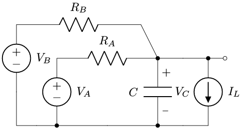
Here we have two voltage sources, \( V_A \) and \( V_B \), a load current \( I_L \), and a capacitor \( C \) with voltage \( V_C \) that is our output. The voltage sources connect to the capacitor via resistances:
- \( R_A \) is an intentional resistance. Let’s just say \( R_A \) = 10KΩ ± 1%.
- \( R_B \) is a parasitic resistance; \( R_B \) = 730KΩ ± 20%.
- \( C \) = 0.11μF ± 5%.
- \( V_A \) is under our control, and is intended to produce a desired waveform across the capacitor.
- \( V_B \) is under our control, but it does something else (not shown in this circuit) and there’s an unavoidable leakage path to the capacitor.
- Both \( V_A \) and \( V_B \) can range anywhere from 0 - 3.3V
- \( I_L \) is an annoying and unpredictable load current:
- it is not under our control
- it varies unpredictably between 0 and 10μA.
- we can’t even observe it directly
- We measure \( V_C \) with a 12-bit analog-to-digital converter.
- Every 100μs we adjust \( V_A \) and \( V_B \) according to some kind of control loop: \( V_A \) to control \( V_C \), and \( V_B \) to control something else.
Now, here’s our problem: we want to improve the control of \( V_C \) by taking into account the effects of component tolerance in \( R_A \), \( R_B \), and \( C \), perhaps by tuning a control loop more aggressively and using feedforward to cancel the effect of \( V_B \) on \( V_C \). Who knows. That’s not the point of this article. In fact, we’re not even going to try to use a control loop in this article; it just makes things more complicated. All we’re going to do here is try to estimate the transfer functions from \( V_A \) to \( V_C \) and from \( V_B \) to \( V_C \). (There’s also a transfer function from \( I_L \) to \( V_C \) but we really don’t care about it.) We know these as a function of the three passive components:
$$\begin{align} V_C &= \frac{1}{1+\tau s}\left(\frac{R_B}{R_A + R_B}V_A + \frac{R_A}{R_A + R_B}V_B - \frac{R_AR_B}{R_A + R_B}I_L\right) \cr \tau &= (R_A || R_B)C = \frac{R_AR_B}{R_A + R_B}C \end{align}$$.
We can view this circuit as the following block diagram:
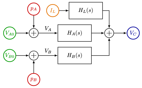
where \( V_{A0} \) and \( V_{B0} \) are the original commands for \( V_A \) and \( V_B \), \( p_A \) and \( p_B \) are the perturbations for \( V_A \) and \( V_B \), and the three transfer functions are
$$\begin{align} H_A(s) &= \frac{\alpha_A}{1+\tau s} \cr H_B(s) &= \frac{\alpha_B}{1+\tau s} \cr H_L(s) &= \frac{-R_L}{1+\tau s} \end{align}$$
with \( \alpha_A = \frac{R_B}{R_A + R_B}, \alpha_B=\frac{R_A}{R_A + R_B}, R_L = \frac{R_AR_B}{R_A + R_B} \).
The nominal values are \( \tau \) = 1085μs and \( V_C = \frac{1}{1+\tau s}\left(0.9865V_A + 0.0135V_B - 9.865K\Omega\cdot I_L\right) \).
Ra = 10e3
Rb = 730.0e3
C = 0.11e-6
tau = 1.0/(1.0/Ra + 1.0/Rb) * C
alpha_A = Rb/(Ra+Rb)
alpha_B = Ra/(Ra+Rb)
R_L = Ra*Rb/(Ra+Rb)
print("tau=%.1fus" % (tau*1e6))
print("alpha_A=%.4f" % alpha_A)
print("alpha_B=%.4f" % alpha_B)
print("R_L=%.3f Kohm" % (R_L/1e3))
tau=1085.1us alpha_A=0.9865 alpha_B=0.0135 R_L=9.865 Kohm
For now, let’s just say that we keep \( V_A = 0.66V = 0.2V_{ref} \) (for \( V_{ref} = 3.3V \)) with no feedback to regulate \( V_C \), and that \( V_B \) is a 5Hz square wave between \( 0.2V_{ref} \) and \( 0.8V_{ref} \).
Let’s set up a simple simulation to show the nominal case:
%matplotlib inline
import numpy as np
import matplotlib.pyplot as plt
from matplotlib import gridspec

def make_adcq(nbits):
    '''
    quantize for adc
    '''
    B = 1.0 / (1 << nbits)
    def adcq(x):
        return np.floor(x/B)*B
    return adcq

def sysid_sim(Ra, Rb, C, pVa, pVb, N, dt=100e-6, seed=None, ilfunc=None):
    '''
    simulation of Ra-Rb-C system

    Ra, Rb, C are component values
    pVa and pVb are perturbation signals to add in to Va and Vb
    N = number of steps

    seed can either be a seed to use with np.random.RandomState,
    or a np.random.RandomState object to handle several successive
    simulations

    Voltages are ratiometric to some Vref somewhere
    '''

    tau = 1.0/(1.0/Ra + 1.0/Rb) * C
    # match discrete (1-alpha)^n to continuous e^(-dt/tau*n)
    alpha = 1-np.exp(-dt/tau)
    alpha_A = Rb/(Ra+Rb)
    alpha_B = Ra/(Ra+Rb)
    R_L = Ra*Rb/(Ra+Rb)
    t = np.arange(N)*dt
    zero = np.zeros(N)

    # in case pVa and pVb are scalars, extend them to a vector
    pVa += zero
    pVb += zero

    # Vb is a square wave between 0.2 and 0.8*Vref
    # with T1 = 1msec

    T1 = 1e-3
    sqwave = (t/(200*T1)) % 1 < 0.5

    Va = np.ones(N) * 0.2 + pVa
    Vb = (1+3*sqwave)/5.0 + pVb
    Vc = np.zeros(N)

    if ilfunc is None:
        il = np.zeros_like(t)
    else:
        il = ilfunc(t, seed=seed)

    vref = 3.3
    Vck = 0

    # Iterative simulation
    for k in xrange(N):

        # find the DC equivalent of VC (if C were 0)
        Vc_dc = alpha_A * Va[k] + alpha_B * Vb[k] - R_L*il[k]/vref
        # now filter it with time constant tau
        Vck += alpha*(Vc_dc - Vck)
        Vc[k] = Vck

    return dict(t=t, Vb=Vb, il=il, Vc=Vc, Va=Va, dt=dt,
                tau=tau, alpha=alpha, alpha_A=alpha_A, alpha_B=alpha_B)

def ilfunc1(t, seed):
    # IL is a value k*2uA where k is a random integer between 0 and 5
    # that changes at random intervals with transition rate alpha_L
    # (total = 0-10uA)

    # Set up PRNG
    if isinstance(seed, np.random.RandomState):
        rs = seed
    else:
        rs = np.random.RandomState(seed=seed)

    alpha_L = 10.0   # average number of transitions/sec
    N = len(t)
    dt = (t[-1] - t[0]) / N
    il_transitions = rs.random_sample(N) < alpha_L*dt
    il_count = np.cumsum(il_transitions)
    il_values = 2e-6 * rs.randint(0, 6, size=il_count[-1]+1)
    il = il_values[il_count]
    return il

S = sysid_sim(Ra=Ra, Rb=Rb, C=C,
              pVa=0,pVb=0,N=20000,seed=1234,
              ilfunc=ilfunc1)
fig = plt.figure(figsize=(7,7))
gs = gridspec.GridSpec(3,1,height_ratios=[1,1,3])

def plot_V_B(S, ax):
    t_msec = S['t']/1e-3
    ax.plot(t_msec,S['Vb'],label='V_B')
    ax.legend(loc='best',labelspacing=0,fontsize=10)
    ax.set_ylim(0,1)
    ax.set_ylabel('V_B/Vref')

def plot_I_L(S, ax):
    t_msec = S['t']/1e-3
    ax.plot(t_msec, S['il']*1e6)
    ax.set_ylabel('I_L (uA)')
    ax.set_ylim(-1,11)

ax = fig.add_subplot(gs[0])
plot_V_B(S, ax)

def plot_V_C_V_A(S, ax):
    t_msec = S['t']/1e-3
    ax.plot(t_msec,S['Vc'],label='V_C')
    ax.plot(t_msec,S['Va'],label='V_A')
    ax.legend(loc='best',labelspacing=0,fontsize=10)
    ax.set_ylabel('V/Vref')

ax2 = fig.add_subplot(gs[1])
plot_I_L(S, ax2)

ax3 = fig.add_subplot(gs[2])
plot_V_C_V_A(S,ax3)
ax3.set_xlabel('t (msec)');
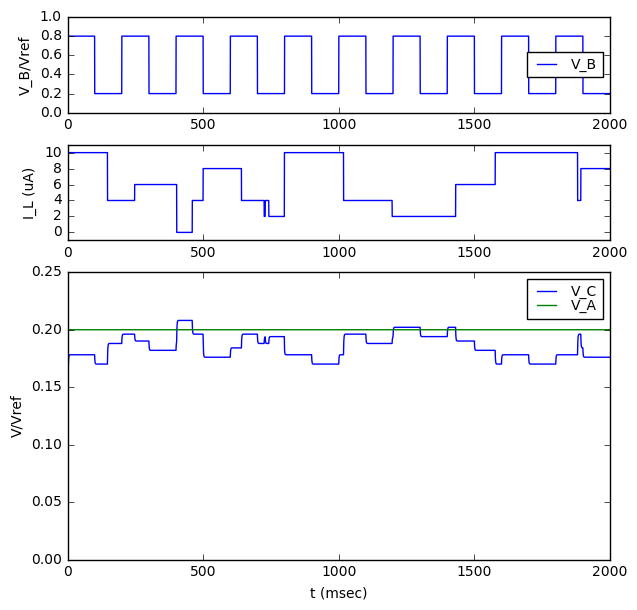
Okay, so that’s mildly interesting. Now let’s try applying some perturbation signals to \( V_A \) and \( V_B \) and see if that can help us understand the transfer functions from A and B to C.
Sinusoidal perturbation
Let’s try using a sinusoidal perturbation signal first. As we’ll see later, this will allow us to probe our system in the frequency-domain, at whatever frequency we use for the perturbation signal.
- Add \( V_{pA} = V_1 \cos \omega t \) as a perturbation signal to \( V_A \)
- Measure \( V_C \) and \( V_A \)
- Compute \( S(V) = \frac{2}{NV_1}\int V e^{-j \omega t}\, dt \) over some integer number \( N \) of full periods, for both \( V_C \) and \( V_A \). (In a discrete-time system, the integral becomes a sum.)
This essentially computes the transfer function of a sine wave input, considered only at that frequency. For example, if \( V_C = V_A = V_{pA} \) then it’s fairly easy to show that \( S_C = S_A =1 \). (dust off your calculus books!)
Also, for a moment we’re going to pretend that we can make perfect measurements with infinite resolution.
N = 20000
dt = 100e-6
t = np.arange(N)*dt
f1 = 100
Nstep = 1.0/(f1*dt)
Nstep_int = int(np.round(Nstep))
f = 1.0/Nstep_int/dt
# actual frequency -- restrict to integer # of steps
# per electrical cycle
theta = 2*np.pi*f*t
c = np.cos(theta)

pVa_amplitude = 0.005
pVb_amplitude = 0
S = sysid_sim(Ra=Ra, Rb=Rb, C=C,
                                  pVa=pVa_amplitude*np.cos(theta),
                                  pVb=pVb_amplitude*np.cos(theta),
                                  N=N,seed=1234,ilfunc=ilfunc1)

fig = plt.figure(figsize=(7,9))
gs = gridspec.GridSpec(3,1,height_ratios=[1,3,1])

ax1 = fig.add_subplot(gs[0])
plot_I_L(S, ax1)

ax2 = fig.add_subplot(gs[1])
plot_V_C_V_A(S, ax2)

def calcS(V,theta,Nstep_int):
    ejth = np.exp(-1j*theta)
    S = np.diff(np.cumsum(ejth*V)[::Nstep_int])/Nstep_int * 2
    return S

S['S_A'] = calcS(S['Va'],theta,Nstep_int)
S['S_C'] = calcS(S['Vc'],theta,Nstep_int)


def plot_S_C_S_A(S, ax):
    t_msec = S['t'] / 1e-3
    ax.set_xlabel('t (msec)');
    for Sx,l in [(S['S_C'],'S_C'), (S['S_A'],'S_A')]:
        ax3.plot(t_msec[::Nstep_int][:-1], np.real(Sx),
             drawstyle='steps', label=l)
    ax.legend(loc='best',labelspacing=0,fontsize=10)

ax3 = fig.add_subplot(gs[2])
plot_S_C_S_A(S, ax3)
ax3.set_ylim(0,0.01);
print "f=%.1fHz (%d steps per cycle)" % (f,Nstep_int)
f=100.0Hz (100 steps per cycle)

We made a 100Hz perturbation of 0.005 amplitude and essentially got what we asked for. The computed amplitudes \( S_A \) and \( S_C \) aren’t very far off from the real amplitudes. The computed amplitude \( S_C \) gets disturbed quite a bit whenever there are large changes in \( V_C(t) \), which makes sense, but it confounds some of our signal processing needs.
So we’re going to do something that’s easy in post-processing on a computer, but difficult to do in real-time on an embedded system — namely compute a robust mean by throwing out the most extreme 10% of the data, hoping that we can get enough “quiet time” to get a good estimate of signal amplitudes:
def robust_mean(x, tail=0.05):
    x = np.sort(x)
    N = len(x)
    Ntail = int(np.floor(N*tail))
    return x[Ntail:-Ntail-1].mean()

def plot_tf_robust(S, ax=None, ref=None, input_key = 'S_A', output_key='S_C'):
    if ax is None:
        fig = plt.figure()
        ax = fig.add_subplot(1,1,1)
    ax.set_xlabel('t (msec)')
    t_msec = S['t']/1e-3
    stats = {}
    for key in [input_key, output_key]:
        Sx = S[key]
        label = key
        line, = ax.plot(t_msec[::Nstep_int][:-1], np.real(Sx),
                 drawstyle='steps', label=label)
        mS = robust_mean(Sx)
        stats[key] = mS
        msg = 'robust mean({0}) = {1:.5f}'.format(label,mS)
        if ref is not None:
            msg += ' = ref*({0:.5f})'.format(mS/ref)
        print msg
        ax.plot([t_msec[0],t_msec[-1]],np.real([mS,mS]),color=line.get_color(),
               alpha=0.25, linewidth=4)
    print "ratio            = {0:.5f}".format(stats[output_key]/stats[input_key])
    ax.legend(loc='best',labelspacing=0,fontsize=10);
    return ax

ax = plot_tf_robust(S, ref=0.005, input_key='S_A', output_key='S_C')
ax.set_ylim(0.0,0.01);
robust mean(S_A) = 0.00500-0.00000j = ref*(1.00000-0.00000j) robust mean(S_C) = 0.00344-0.00218j = ref*(0.68807-0.43624j) ratio = 0.68807-0.43624j

The robust-mean algorithm works fairly well to filter out those spikes; in the graph above, the thick transparent lines are the robust mean. For \( V_A \), which has the computed amplitude 0.005, just what our perturbation signal is, we get a detected amplitude that is exactly what we applied as an input. For \( V_C \) we’re getting the perturbation amplitude 0.005 times (0.68807-0.43624j). The actual value of the transfer function is \( \alpha_A / (1 + \tau s) \) with \( \alpha_A = 0.9865 \) and \( \tau = \) 326μs. Let’s evaluate at \( s = 2\pi jf \) for \( f=100 \) Hz:
print ('Actual transfer function at f={0:.1f}Hz: {1:.5f}'.format(
        f, alpha_A / (1 + tau * 2j * np.pi * f)))
Actual transfer function at f=100.0Hz: 0.67343-0.45915j
Hmm. Not quite the same as what we measured.
Now let’s put the ADC back into the picture and look at what happens when the input is quantized:
for resolution in [12, 10]:
    print "ADC resolution = %d:" % resolution
    adcq = make_adcq(resolution)
    S['S_A'] = calcS(adcq(S['Va']),theta,Nstep_int)
    S['S_C'] = calcS(adcq(S['Vc']),theta,Nstep_int)
    ax = plot_tf_robust(S, ref=0.005, input_key = 'S_A', output_key = 'S_C')
    ax.set_title('Sine-wave amplitude estimation with %d-bit ADC' % resolution)
    ax.set_ylim(0.0,0.01);
ADC resolution = 12: robust mean(S_A) = 0.00500-0.00000j = ref*(1.00084-0.00000j) robust mean(S_C) = 0.00344-0.00218j = ref*(0.68779-0.43578j) ratio = 0.68721-0.43541j ADC resolution = 10: robust mean(S_A) = 0.00496-0.00000j = ref*(0.99169-0.00000j) robust mean(S_C) = 0.00344-0.00217j = ref*(0.68726-0.43485j) ratio = 0.69301-0.43849j
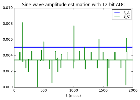

Yeah, the ADC resolution matters here. Look at those little shifts in the S_C waveform in the 10-bit ADC case, which are barely perceptible in the 12-bit ADC case. Real systems don’t do so well with detecting signals that aren’t that large compared to the ADC resolution.
Now let’s try doing this at a number of different frequencies:
def sysid_probe_1(dt, N, freqlist=[2.8,5,7,10,14,20,28,50,70,100,140,200,280,500],
                  seed=None,ilfunc=None,verbose=False,ntrials=1):
    t = np.arange(N)*dt
    tflist = {}
    rs = np.random.RandomState(seed) if seed is not None else None
    for which in ['A', 'B']:
        if verbose:
            print 'Perturbing V_%s' % which
        tflist[which] = []
        if which == 'A':
            pVa_amplitude = 0.005
            pVb_amplitude = 0
            lwhich = 'Va'
        else:
            pVb_amplitude = 0.005
            pVa_amplitude = 0
            lwhich = 'Vb'
        for f1 in freqlist:
            Nstep = 1.0/(f1*dt)
            Nstep_int = int(np.round(Nstep))
            f = 1.0/Nstep_int/dt
            # actual frequency -- restrict to integer # of steps
            # per electrical cycle
            theta = 2*np.pi*f*t
            c = np.cos(theta)

            data = [f1]

            for itrial in xrange(ntrials):
                if verbose:
                    print "trial #%d" % (itrial+1)
                S = sysid_sim(Ra=Ra, Rb=Rb, C=C,
                                                  pVa=pVa_amplitude*np.cos(theta),
                                                  pVb=pVb_amplitude*np.cos(theta),
                                                  N=N,seed=rs,ilfunc=ilfunc)

                for k in 'a b c'.split():
                    V = S['V'+k]
                    Sx = calcS(V,theta,Nstep_int)
                    S['S'+k] = Sx
                k = 'Sa' if which == 'A' else 'Sb'
                Sx = S[k]
                Sy = S['Sc']
                H = robust_mean(Sy)/robust_mean(Sx)
                if verbose:
                    print 'f={0:5.1f}: Sc/{1}={2:.4f}'.format(f1, k, H)
                data.append(H)
            tflist[which].append(data)
        tflist[which] = np.array(tflist[which])
    return tflist

def plot_tflist(tflist, dt, N, ntrials=1):
    fig = plt.figure()
    ax = fig.add_subplot(1,1,1)
    f1 = np.logspace(0,3,1000)
    legend_handles = []
    for which,color,marker in [('A','red','.'), ('B','green','x')]:
        tfdata = tflist[which]
        f = np.abs(tfdata[:,0])
        H_est = tfdata[:,1:]
        H_est_dB = 20*np.log10(np.abs(H_est))
        H_theoretical = (alpha_A if which == 'A' else alpha_B)/(1+tau*2j*np.pi*f1)
        H_theo_dB = 20*np.log10(np.abs(H_theoretical))
        ax.semilogx(f1,H_theo_dB,linewidth=0.5,color=color)
        h = ax.semilogx(f,H_est_dB,marker, color=color)
        legend_handles.append(h[0])
    ax.set_title('Detected and theoretical amplitudes from sine-wave system ID'
                 +'\n(%d samples at %.1fkHz for each data point, %d %s)'
                   % (N, 0.001/dt, ntrials, 'trials' if ntrials > 1 else 'trial'),
                fontsize=10)
    ax.legend(labels=['A','B'],handles = legend_handles, loc='best')
    ax.set_xlabel('f (Hz)')
    ax.set_ylabel('|H_est(f)| (dB)')
    ax.grid('on')
    ax.set_ylim(-60,10)

N = 10000
ntrials = 5
dt = 100e-6
tflist = sysid_probe_1(dt,N,seed=1234,ilfunc=ilfunc1,ntrials=ntrials)
plot_tflist(tflist, dt, N, ntrials)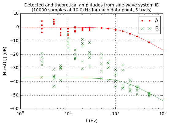
Now we’re seeing a better picture here. The sine-wave system ID doesn’t do a bad job, at least at the higher frequencies and with \( H_A(s) \). There’s very good matching with the theoretical transfer function. At low frequencies, what’s happening is that there is energy from other unwanted signals, and there’s no way to separate out that unwanted frequency content from the information we actually want to measure, which is the amplitude and phase of the perturbation signal that makes it through from input to output. Also, it takes a lot of time to get this data: each plot point in the above graph represents probing using a different frequency sine wave (14 different frequencies in the plot above), so to get the all data points we really had to take 280,000 different samples. (10000 samples × 14 test frequencies × 2 perturbation paths, A → C and B → C)
(The \( H_B(s) \) transfer function has higher relative error, because it’s a much smaller signal. Maybe we don’t need to know it precisely; maybe we do.)
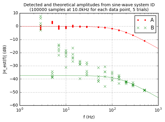
We could do better estimating both transfer functions by taking even more samples, of course, so that the unwanted signals average out. Let’s bump things up by a factor of 10, for 2.8 million samples total. Note that this is going to take 280 seconds worth of data at 10kHz sampling rate, but we’d really like to get a good estimate of the transfer function:
N = 100000
ntrials = 5
dt = 100e-6
tflist = sysid_probe_1(dt,N,seed=1234,ilfunc=ilfunc1,ntrials=ntrials)
plot_tflist(tflist,dt,N,ntrials)
Now let’s change our test system a little bit by using a different load current \( I_L \). It’s still going to be 0-10μA, but this time we’re going to make it a frequency-modulated sine wave in the 182-222Hz range.
import scipy.signal

def ilfunc2(t, seed):
    # IL is a 0-10uA, frequency-modulated sine-wave
    # with frequency content ranging roughly from 182-222Hz.

    # Set up PRNG
    if isinstance(seed, np.random.RandomState):
        rs = seed
    else:
        rs = np.random.RandomState(seed=seed)

    fcarrier = 202
    fspread = 20

    tau = 0.02
    alpha = dt/tau
    fp = 2*np.pi*rs.randn(*t.shape)
    fpfilt = scipy.signal.lfilter([alpha],[1.0, alpha-1.0],fp)
    tmod = t+1.0*fspread/fcarrier*np.cumsum(dt*fpfilt)
    theta = 2*np.pi*fcarrier*tmod

    il = 10e-6 * (1+np.sin(theta))/2

    return il
df = 1/(t[-1]-t[0])
ilsample = ilfunc2(t,seed=1234)
ilspectrum = 20*np.log10(np.abs(np.fft.fft(ilsample)))
for k, nf in enumerate([len(ilspectrum)//2, 1000]):
fig = plt.figure(figsize=(6,10))
ax = fig.add_subplot(2,1,k+1)
ax.plot(np.arange(nf)*df, ilspectrum[:nf])
ax.grid('on')
ax.set_title('FFT-computed spectrum of ilfunc2()')
ax.set_ylabel('|I_L| (dB)')
ax.set_xlabel('f (Hz)');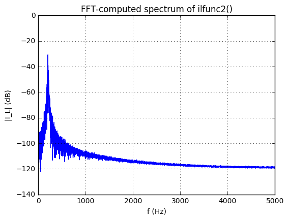

OK, now let’s run our test simulation with a sine-wave perturbation and using the 202Hz-centered ilfunc2 for the load current \( I_L \):
N = 100000
ntrials=5
dt = 100e-6
tflist = sysid_probe_1(dt,N,seed=1234,ilfunc=ilfunc2,ntrials=ntrials)
plot_tflist(tflist,dt,N,ntrials=ntrials)

It works great… except at the 200Hz point we get a bunch of noise.
Correlating a measured output with a sine-wave perturbation signal is very useful. You can essentially read off the transfer function directly from each frequency used. The only issue is that there’s no way to distinguish the response from the perturbation frequency and the system’s normal content at that frequency.
System Identification with Spread-Spectrum Perturbation
Now we’re going to use the output from an LFSR as a perturbation signal. This acts as a pseudorandom bit sequence (PRBS) or pseudonoise (PN) sequence. We talked about the correlation properties of an LFSR-based PRBS in part XI, but let’s recap and be a little more careful. The cross-correlation \( R_{xy}[\Delta k] \) between any two repeating signals \( x[k] \) and \( y[k] \) with period \( n \) is defined as
$$R _ {xy}[\Delta k] = \sum\limits_{k=0}^{n-1} x[k]y[k-\Delta k] $$
where the index \( k-\Delta k \) wraps around because of the repeating signals. (For nonrepeating signals, the limits of the sum are from \( -\infty \) to \( \infty \).)
We’re going to use a cross-correlation normalized to the number of samples:
$$C _ {xy}[\Delta k] = \tfrac{1}{n}R _ {xy}[\Delta k] = \tfrac{1}{n}\sum\limits_{k=0}^{n-1} x[k]y[k-\Delta k] $$
If \( y[k] = x[k] \) then we can calculate \( C_{xx}[\Delta k] \) as the autocorrelation. If you remember from part XI, the correlation between the output of a maximum-length LFSR \( b[k] \) with values scaled to ±1, and any delayed version of that same output, is
$$C_{bb}[\Delta k] = \tfrac{1}{n}\sum\limits_{k=0}^{n-1} b[k]b[k-\Delta k] = \begin{cases} 1 & \Delta k = 0 \cr -\frac{1}{n} & \Delta k \ne 0 \end{cases}$$
for \( n=2^N - 1 \) in the case of an LFSR with primitive polynomial. (This two-valued behavior, where the correlation is close to zero for \( \Delta k \ne 0 \), is very useful, and we’ll make use of it in a bit.)
We can also find the cross-correlation \( C_{by}[\Delta k] \) between \( b[k] \) and some other signal \( y[k] \). So if we use \( b[k] \) as a perturbation signal, we can correlate the system response \( y[k] \) with \( b[k] \), calculating \( C_{by}[\Delta k] \). If \( \Delta k = 0 \) then result will essentially tell us how much of the system response has no delay. Then we can correlate the system response with \( b[k-1] \) to find \( C_{by}[1] \) and the result will tell us how much of the system response has a delay of 1 step. Repeat and we can get the whole time-domain response of the transfer function.
Huh?
Okay, let’s take that a little more slowly. Below is a plot of the first 200 samples of one LFSR’s output \( b[k] \), and we’re going to correlate it with various signals:
- \( b[k] \) (to show correlation of 1)
- time-shifted versions \( b[k-\Delta k] \)
- a repeating sequence of ones (to show correlation with the DC component of any signal)
- a random sequence of ±1
from libgf2.gf2 import GF2QuotientRing, checkPeriod

def lfsr_output(field, initial_state=1, nbits=None):
    n = field.degree
    if nbits is None:
        nbits = (1 << n) - 1
    u = initial_state
    for _ in xrange(nbits):
        yield (u >> (n-1)) & 1
        u = field.lshiftraw1(u)

f18 = GF2QuotientRing(0x40027)
assert checkPeriod(f18,262143) == 262143

pn18 = np.array(list(lfsr_output(f18))) * 2 - 1
fig = plt.figure(figsize=(6,2))
ax = fig.add_subplot(1,1,1)
ax.plot(pn18[:200],'-',drawstyle='steps')
ax.set_ylim(-1.1,1.1);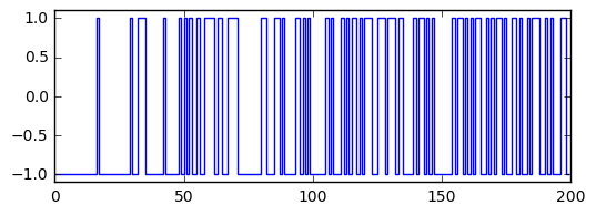
n=len(pn18)

def pncorrelate(x, pn):
    return np.sum(x*pn)*1.0/len(pn)

print "n=%d" % n
print "1/n=%g" % (1.0/n)
print "Pseudonoise correlation with various signals:"
print "self:              ", pncorrelate(pn18,pn18)
for delta_k in xrange(1,5):
    print "self shifted by %d: %g" %(delta_k, pncorrelate(np.roll(pn18,delta_k),pn18))
print "ones:               %g" % pncorrelate(np.ones(len(pn18)), pn18)
ntry = 1000
print "%d random trials (first 10 shown):" % ntry
np.random.seed(123)
clist = []
for itry in xrange(ntry):
    c = pncorrelate(np.random.randint(2, size=n)*2-1, pn18)
    if itry < 10:
        print "random +/-1: %8.5f" % c
    clist.append(c)
print "std dev: %.5f (%.5f expected)" % (np.std(clist), 1.0/np.sqrt(n))
n=262143 1/n=3.81471e-06 Pseudonoise correlation with various signals: self: 1.0 self shifted by 1: -3.81471e-06 self shifted by 2: -3.81471e-06 self shifted by 3: -3.81471e-06 self shifted by 4: -3.81471e-06 ones: 3.81471e-06 1000 random trials (first 10 shown): random +/-1: -0.00584 random +/-1: 0.00177 random +/-1: -0.00106 random +/-1: 0.00138 random +/-1: 0.00003 random +/-1: -0.00239 random +/-1: 0.00004 random +/-1: -0.00051 random +/-1: -0.00154 random +/-1: 0.00094 std dev: 0.00197 (0.00195 expected)
OK, great! We already talked about the autocorrelation \( C_{bb}[\Delta k] \), and sure enough we get 1 for \( \Delta k=0 \) and \( -1/n \) for a few values of \( \Delta k > 0 \).
The cross-correlation of a PRBS with a sequences of ones is \( 1/n \).
The cross-correlation of a PRBS with a random sequence of ±1 bits is a random variable that is approximately a normal distribution with zero mean and standard deviation of \( 1/\sqrt{n} \).
This \( 1/\sqrt{n} \) behavior is pretty common whenever we try to “defeat” the randomness of random noise by taking more and more samples. Yes, you can cut the amplitude by a factor of 2, but to do so you need to increase the number of samples by a factor of 4.
Anyway, now let’s use our PRBS for system identification:
def pncorrelate_array(x,y,karray):
return np.array([pncorrelate(x,np.roll(y,k)) for k in karray])
def pn_sysid(pn,karray,ilfunc=ilfunc1,
input_signal='Va', output_signal='Vc',
input_amplitude=pVa_amplitude,
filter=None):
perturbation = input_amplitude*pn
S = sysid_sim(Ra=Ra, Rb=Rb, C=C,
pVa=perturbation if input_signal == 'Va' else 0,
pVb=perturbation if input_signal == 'Vb' else 0,
N=len(pn),seed=1234,ilfunc=ilfunc)
if filter is None:
filter = lambda x: x
Cin = pncorrelate_array(filter(S[input_signal]),pn,[0])
Cout = pncorrelate_array(filter(S[output_signal]),pn,karray)
return Cout, Cin, S
def correlation_waveforms(Cc, Ca, pn, field, karray, h, fig=None):
kmin = min(karray)
kmax = max(karray)
k_theo = np.linspace(kmin,kmax,10000)
if fig is None:
fig = plt.figure(figsize=(6.8,4))
ax=fig.add_subplot(1,1,1)
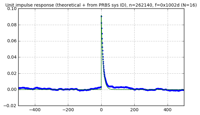
ax.set_title('Unit impulse response (theoretical + from PRBS sys ID), '+
'n=%d, f=0x%x (N=%d)' % (len(pn), field.coeffs, field.degree), fontsize=10)
ax.plot(karray,Cc/Ca[0],'.')
if h is not None:
ax.plot(k_theo,h(k_theo))
ax.set_xlim(kmin,kmax)
ax.grid('on')
kmax = 500
karray = np.arange(-kmax, kmax)
Cc, Ca, S = pn_sysid(pn18,karray)
def h_theoretical(k,A=1.0):
alpha = dt/tau
kpos = k*(k>=0)
return A*alpha*np.exp(-kpos*alpha)*(k>=0)
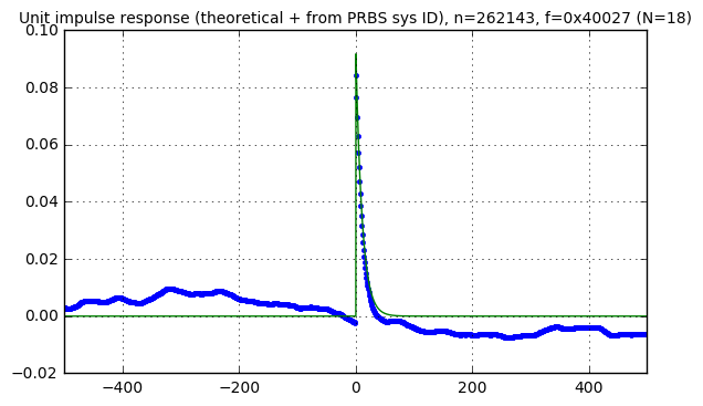
correlation_waveforms(Cc,Ca,pn18,f18,karray, h_theoretical)
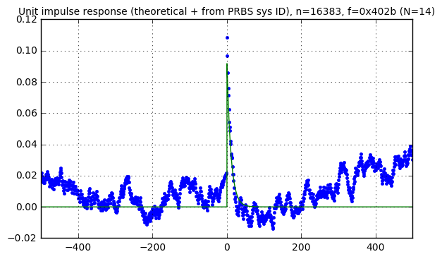
Now that’s interesting. We do get a very nice response using PRBS for system ID, that looks like the impulse response, but it is shifted upwards with some noisy content. That noisy offset is essentially the energy in the undisturbed system output, scrambled in the frequency domain to be spread over the spectrum of the PRBS.
Why do we get the impulse response? The two-valued autocorrelation \( C_{bb}[\Delta k] = 1 \) for \( \Delta k = 0 \) and \( C_{bb}[\Delta k] = -1/n \approx 0 \) for \( \Delta k \ne 0 \) means that the set of delayed PRBS sequences \( b[k-\Delta k] \) can be used as a quasi-orthonormal basis. (A true orthonormal basis would have cross-correlation of 1 between identical signals and 0 between different signals.) And because our system is linear time-invariant, the output response \( y[k] \) we’re trying to analyze (for example, \( y = V_C \)) can be written as the following superposition over each possible delay \( \Delta k \):
$$\begin{align} y[k] &= y_0[k] + \sum\limits_{\Delta k = 0}^{n-1} b[k-\Delta k]h[\Delta k] \cr &= \sum\limits_{\Delta k = 0}^{n-1} b[k-\Delta k]\left(h[\Delta k] + Y_0[\Delta k]\right) \end{align}$$
where
- \( y_0[k] \) is the output that we would have observed if we hadn’t perturbed the input
- \( Y_0[\Delta k] \) is \( y_0[k] \) decomposed into components weighting \( b[k-\Delta k] \)
- each \( h[\Delta k] \) component is one sample of the impulse response.
If you think this looks similar to a Fourier transform, you’re right! Fourier transforms are only one example of the use of an orthonormal basis. Anytime you have signals with two-valued autocorrelation where the \( \Delta k = 0 \) term has correlation of 1, and the \( \Delta k \ne 0 \) term has correlation of 0, it has many properties similar to a Fourier transform, such as the decomposition into weighted sums of basis components, preservation of energy (Parseval’s theorem), etc. And so we have the Hadamard-Walsh transform which uses square-wave-like basis functions (the Walsh functions). The PRBS from an LFSR doesn’t have exactly zero correlation for \( \Delta k \ne 0 \), so it’s not quite a perfect orthonormal basis, but it’s close enough for large \( n \). (And those of you who are nitpicky linear algebra students can fix the errors in your spare time, using orthogonalization techniques. Have at it!)
What about the noise? We’ll talk about that in just a minute.
For now let’s step back for a second and look at the big picture.
System Identification — the Big Picture
System identification has a few major aspects, including:
- Creating a proposed model of the unknown part(s) of the system — maybe our model is a transfer function of known structure with unknown parameters like \( H(s) = 1/(\tau s + 1) \), or maybe it falls into one of many systematic approaches like ARMA or ARMAX
-
Experiment design — one of the terms used in this field; system ID is essentially running an experiment on a system to gain information about it. Experiment design involves determining things like
- what kinds of input disturbance signals to use
- how large of an amplitude should be used as a disturbance
- whether passive identification is sufficient
- how many samples to take
- how often to sample
- whether pre- or post-filtering is helpful
- how to handle closed-loop control systems
-
Implementing and executing the experiment
- Analyzing the results to estimate model parameters and their uncertainty
The core idea of using sine waves or PRBS as input disturbance signals is fairly simple, and as we’ve seen, using sine waves gets us samples of the transfer function in the frequency domain, whereas PRBS gives us samples of the impulse response in the time domain. But that’s only the beginning, and a whole bunch of other issues need to be resolved, before you can actually get system identification working reliably. As I said before, I’m not an expert, so I don’t have answers for a lot of them, and there aren’t many books or articles that are written with the generalist engineer in mind; you have to be willing to wade through a bunch of equations to get somewhere useful.
Having said that, here are a few other practical thoughts:
Reflected Pseudonoise
Look at the last graph we drew here. It’s an impulse response with a noisy offset. I’m going to call it “reflected pseudonoise”, for reasons that may become clear later. Where does this noise come from, and how do we deal with it when we interpret the results?
Each of our estimates has some uncertainty, and the trick is being able to understand where the uncertainty comes from, in order to estimate how large the uncertainty is, and then determine how much of an impact that uncertainty has when we use those results.
For some kinds of measurements, this is fairly easy. Got an ADC input? If you have an ADC channel that is connected to a known constant voltage, you can get the uncertainty empirically by taking a bunch of samples and computing the standard deviation. Or you can bound the errors by checking the datasheets for the ICs you are using, and come up with worst-case bounds; this is usually much more conservative than using statistical measurements.
But computing uncertainty for derived calculations is difficult. What we’d like to do is try some things and see if we can justify an empirical relationship between aspects of our system and the parameter uncertainties — for example, maybe the amplitude of that noisy offset is closely correlated with the amplitude of the disturbance signal and the number of samples used.
Let’s do some experiments and look at some empirical observations.
We should expect the noisy offset to change with the period of the PRBS, so let’s try using a 12-bit, a 14-bit, and a 16-bit PRBS:
f12 = GF2QuotientRing(0x1053)
p12 = (1<<12) - 1
assert checkPeriod(f12,p12) == p12

pn12 = np.array(list(lfsr_output(f12))) * 2 - 1

kmax = 500
karray = np.arange(-kmax, kmax)
Cc, Ca, S = pn_sysid(pn12,karray)
correlation_waveforms(Cc,Ca,pn12,f12,karray,h_theoretical)

f14 = GF2QuotientRing(0x402b)
p14 = (1<<14) - 1
assert checkPeriod(f14,p14) == p14

pn14 = np.array(list(lfsr_output(f14))) * 2 - 1

kmax = 500
karray = np.arange(-kmax, kmax)
Cc, Ca, S = pn_sysid(pn14,karray)
correlation_waveforms(Cc,Ca,pn14,f14,karray,h_theoretical)
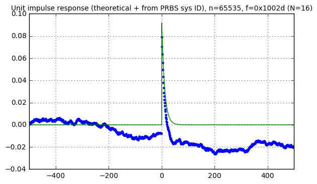
f16 = GF2QuotientRing(0x1002d)
p16 = (1<<16) - 1
assert checkPeriod(f16,p16) == p16

pn16 = np.array(list(lfsr_output(f16))) * 2 - 1

kmax = 500
karray = np.arange(-kmax, kmax)
Cc, Ca, S = pn_sysid(pn16,karray)
correlation_waveforms(Cc,Ca,pn16,f16,karray,h_theoretical)
Now that’s not really fair; the smaller-size LFSRs have shorter periods, and if we use less samples from the signals in our system, we’re bound to get a poorer response. So let’s try to normalize and use approximately \( 2^{18} \) samples in each case:
def pnr(field, n=None):
    """ pseudonoise, repeated to approx 2^n samples """
    n0 = field.degree
    if n is None:
        n = n0
    nbits = ((1<<n0)-1) * (1<<(n-n0))
    return np.array(list(lfsr_output(field, nbits=nbits))) * 2 - 1

pn12 = pnr(f12, 18)

kmax = 500
karray = np.arange(-kmax, kmax)
Cc, Ca, S = pn_sysid(pn12,karray)
correlation_waveforms(Cc,Ca,pn12,f12,karray,h_theoretical)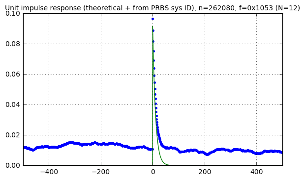
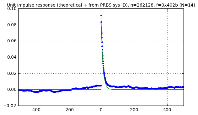
pn14 = pnr(f14, 18)

kmax = 500
karray = np.arange(-kmax, kmax)
Cc, Ca, S = pn_sysid(pn14,karray)
correlation_waveforms(Cc,Ca,pn14,f14,karray,h_theoretical)
pn16 = pnr(f16, 18)

kmax = 500
karray = np.arange(-kmax, kmax)
Cc, Ca, S = pn_sysid(pn16,karray)
correlation_waveforms(Cc,Ca,pn16,f16,karray,h_theoretical)
The response looks sort of the same in all cases, kind of like a random walk, but it’s not clear where this comes from. First let’s make one small change: in order to see the noise without the system response, we’ll run the same experiment as the graph above (approximately \( 2^{18} \) samples with a 16-bit LFSR) but use a disturbance signal of essentially zero:
kmax = 500
def pn_sysid_nodisturbance(pn, karray, ilfunc=ilfunc1):
# same as pn_sysid() but with no disturbance
S = sysid_sim(Ra=Ra, Rb=Rb, C=C,
pVa=0,
pVb=0,
N=len(pn),seed=1234,ilfunc=ilfunc)
Cc = pncorrelate_array(S['Vc'],pn,karray)
Ca = [pVa_amplitude] # amplitude which we were using in pn_sysid()
return Cc, Ca, S
def rms(y):
""" root-mean-square """
return np.sqrt(np.mean(y**2))
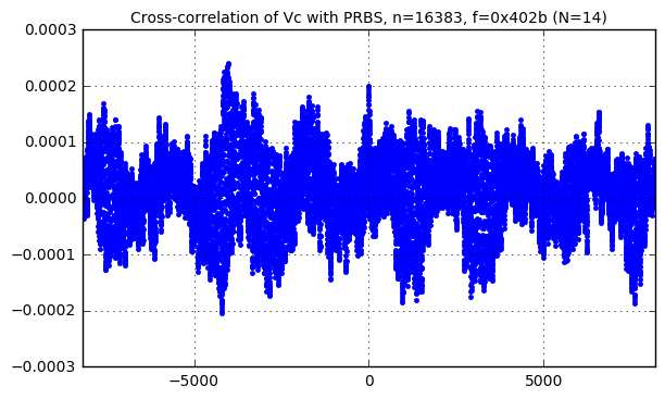
def crosscorr_title(ax, pn, f):
ax.set_title('Cross-correlation of Vc with PRBS, n=%d, f=0x%x (N=%d)'
% (len(pn), f.coeffs, f.degree), fontsize=10)
karray = np.arange(-kmax,kmax)
Cc, Ca, S = pn_sysid_nodisturbance(pn16, karray)
correlation_waveforms(Cc,[1.0],pn16,f16,karray,h=None)
crosscorr_title(plt.gca(), pn16, f16)
Vcmean = S['Vc'].mean()
print "mean(Vc) = ", Vcmean
print "rms(Vc) = ", rms(S['Vc']-Vcmean)
print "pVa_amplitude=", pVa_amplitudemean(Vc) = 0.189627738772 rms(Vc) = 0.0110564161443 pVa_amplitude= 0.005

Okay, remember, we’re computing \( C_{by}[\Delta k] = \tfrac{1}{n}\sum\limits_{k=0}^{n-1}b[k]y_0[k-\Delta k] \) where \( b[k] \) is our pseudonoise waveform, and \( y_0[k] \) is the normal system signal without any perturbation: in this case, it’s the voltage \( V_C \) on the capacitor in the system we’re trying to identify.
Now, \( b[k] \) is our PRBS, which is always ±1 but looks like noise, relative to the signal, and it has a mean value of \( 1/(2^N-1) \) (very close to zero) and standard deviation of 1.0. Statistically, we can think of it as a sequence of independent identically-distributed random variables, which have these properties (in case you don’t remember your probability and statistics course):
- If \( b[k] \) has zero mean and standard deviation \( \sigma \) for all \( k \), and \( a \) is a constant, then \( ab[k] \) has zero mean and standard deviation \( a\sigma \)
- If \( b[k] \) has zero mean and standard deviation \( \sigma \) for all \( k \), then \( a_0b[0] + a_1b[1] + a_2b[2] + \ldots \) has zero mean and standard deviation \( \sigma \sqrt{a_0^2 + a_1^2 + a_2^2 + \ldots} \) — the amplitudes add in quadrature
- Even though \( b[k] \) isn’t Gaussian (it’s a discrete Bernoulli variable), computing large sums like \( a_0b[0] + a_1b[1] + a_2b[2] + \ldots \) tend to have a Gaussian distribution because of the central limit theorem
So we should expect that \( C_{by}[\Delta k] \), when \( b \) and \( y \) are independent, acts somewhat like a Gaussian random variable with close-to-zero mean and standard deviation \( \sigma_C \) as follows:
$$\begin{align} \sigma_C &= \frac{1}{n}\sqrt{\sum\limits_{k=0}^{n-1}y[k]^2} \cr &= \frac{1}{\sqrt{n}}\cdot\sqrt{\frac{1}{n}\sum\limits_{k=0}^{n-1}y[k]^2} \cr &= \frac{1}{\sqrt{n}}\cdot y_{\text{RMS}} \end{align}$$
In other words, the correlation has a bell-curve distribution with standard deviation proportional to the factor \( \tfrac{1}{\sqrt{n}} \) and to \( y_{\text{RMS}} \), the root-mean-square of the input sample data \( y[k] \). If we let \( n \) get really large, this term goes to zero, but with finite \( n \) we’re left with some residual noise. The noise has two components of interest:
- a mean value \( \bar{y} \) (approximately 0.19V in the case of the \( V_C \) waveform)
- RMS \( \sigma_y \) excluding the mean (approximately 0.011V for \( V_C \))
Why is it important to consider these separately? Because they have different gains: the PRBS has a nonzero mean of \( 1/(2^N-1) \) (where \( N \) is the bit size of the LFSR), so the correlation effectively creates a gain of the mean of \( 1/(2^N-1) \), whereas the correlation gain of the RMS component is \( 1/{\sqrt{n}} \) (where \( n \) is the number of samples taken).
In the case shown above, \( N=16 \) and \( n=4\cdot(2^{16}-1) \approx 2^{18} \), so we should expect noise that has a mean of roughly \( 2^{-16}\bar{y} \approx 2.90 \times 10^{-6} \) and a standard deviation of roughly \( 2^{-9}\sigma_y \approx 2.15 \times 10^{-5} \). This is in the same ballpark as the cross-correlation graph above, where the noise wanders around between 1-2 × 10⁻⁵.
The head-scratching part of this comes with the random-walk similarity. If we calculate \( C_{by}[\Delta k] \) and \( C_{by}[\Delta k + 1] \), they tend to be similar. The individual samples \( C_{by}[\Delta k] \) aren’t independent noise sources. What’s going on?
PRBS as an Orthonormal Basis
The answer comes when we consider PRBS as an orthonormal basis, and cross-correlation as a way to transform individual samples \( y_0[k] \) (remember, we’re using the 0 subscript to denote the signal without any perturbation input) into the “PRBS domain” as weighted coefficients \( Y_0[\Delta k] \). This is the reason I call it “reflected pseudonoise”, because it’s the unmodified signals \( y_0[k] \) transformed, or reflected, into “noise” by the operation of correlation.
Perhaps you’re acquainted enough with linear algebra that this idea makes sense. If not, let’s take another look. I’m going to use one of the shorter PRBS runs just to keep the computational load down to a reasonable number.
Here’s the “noise” seen in the cross-correlation from the first 16383 samples of Vc, with the PRBS from a 14-bit LFSR, and this time we’re going to compute all 16383 cross-correlation values:
pn14s = pnr(f14)    # no repeats
kmax = 8192
karray = np.arange(-kmax+1, kmax)
Cc, Ca, S = pn_sysid_nodisturbance(pn14s, karray)
correlation_waveforms(Cc,[1.0],pn14s,f14,karray,h=None)
crosscorr_title(plt.gca(), pn14s, f14)

Now, one interesting aspect of correlating signals with a full period of LFSR output relates to the frequency domain.
Just as the convolution \( x * y \) in the time domain shows up as the product \( X(f)Y(f) \) in the frequency domain, following the Convolution Theorem, the correlation \( C_{xy} \) in the time domain shows up as \( X(f)\bar{Y}(f) \) in the frequency domain, where the bar over the Y is the complex conjugate, due to the Cross-Correlation Theorem. (There’s a nice explanation of this on dsp.stackexchange by Jason R, who is not me.)
What this means is that if we know the Fourier transforms of two signals X and Y, we can calculate the Fourier transform of their correlation without actually calculating the correlation itself. Equivalently, if we want to calculate all possible values of the correlation sequence, we can use FFTs to speed up the calculation.
It gets even more interesting when you correlate with the PRBS from an LFSR, because we showed in part XII that the FFT of a PRBS has uniform amplitude:
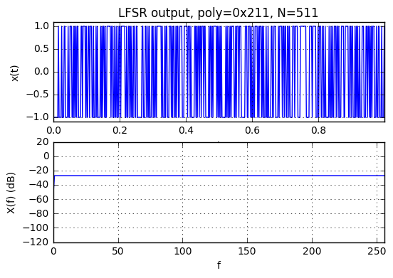
Actually, the fine print is that the FFT is two-valued, but uniform over all frequencies except for DC:
$$\left|B(f)\right| = \begin{cases} 2^{N/2} & f \ne 0 \cr 1 & f = 0 \end{cases}$$
You can just barely see the dip at \( f=0 \) in the graph above, where the amplitude is shown in dB relative to the number of samples N.
The phase of the PRBS in the frequency domain, on the other hand, skips around seemingly randomly, with no discernable pattern.
So the key insight is that because of this weird uniform-amplitude property of the PRBS, and the Correlation Theorem, when you correlate some signal \( y[k] \) with an LFSR-based PRBS \( b[k] \), with an integral number of periods of the LFSR, then the frequency spectrum of the correlation \( C_{by}[\Delta k] \) has the same shape of amplitude (except for a relative attenuation at DC) as the frequency spectrum of \( y[k] \). The phase is scrambled, but the shape of the amplitude is left alone. We essentially get noise with the same power spectral density shape as the spectrum of the original signal. (The scaling is by \( 2^{N/2} \) if the correlation is raw, and approximately \( 2^{-N/2} \) if the correlation is normalized by a factor of \( 1/n=1/(2^N-1) \).)
Don’t believe me? Let’s try it!
# Code from part XI
# https://www.embeddedrelated.com/showarticle/1124.php

def show_fft(x, t=None, fig=None, style='-',
             hide_upper_half=False, upper_half_as_negative=False,
             dbref=None, **kwargs):
    if fig is None:
        fig = plt.figure()
    N = len(x)

    ylim = kwargs.pop('ylim',None)
    freq_only = kwargs.pop('freq_only',False)

    if t is None:
        # support for pandas Series objects
        try:
            t = x.index
        except AttributeError:
            # fallback
            t = np.arange(N)
    if freq_only:
        ax_time = None
        ax_freq = fig.add_subplot(1,1,1)
    else:
        ax_time = fig.add_subplot(2,1,1)
        ax_freq = fig.add_subplot(2,1,2)
    X = np.fft.fft(x)

    if not isinstance(style, basestring) and len(style) == 2:
        tstyle, fstyle = style
    else:
        tstyle = fstyle = style


    if ylim is None:
        xmin = min(x)
        xmax = max(x)
        xspan = xmax-xmin
        ylim = (xmin-xspan*0.05, xmax+xspan*0.05)

    if not freq_only:
        ax_time.plot(t,x,tstyle,**kwargs)
        ax_time.set_xlim(min(t),max(t))
        ax_time.set_ylim(ylim)

    delta_t = t[-1]-t[0]  # this assumes equal spacing....
    df = 1/delta_t
    f = np.arange(N)*df
    if upper_half_as_negative:
        f[f/df>N/2] -= N*df
    if dbref is None:
        ax_freq.plot(f,np.abs(X),fstyle, **kwargs)
        ax_freq.set_ylim(0,np.abs(X).max()*1.05)
    else:
        ax_freq.plot(f,20*np.log10(np.abs(X)*1.0/dbref),fstyle, **kwargs)
        ax_freq.set_ylim(-120,20)
    if hide_upper_half:
        ax_freq.set_xlim(0,N*df/2)
    elif upper_half_as_negative:
        ax_freq.set_xlim(-N*df/2,N*df/2)
    else:
        ax_freq.set_xlim(0,N*df)

    return ax_time, ax_freq

def show_fft_real(x,t=None,**kwargs):
    ax_time, ax_freq = show_fft(x,t,hide_upper_half=True,**kwargs)
    if ax_time is not None:
        ax_time.set_ylabel('x(t)')
        ax_time.set_xlabel('t')
        ax_time.grid('on')

    if 'dbref' in kwargs and kwargs['dbref'] is not None:
        ax_freq.set_ylabel('X(f) (dB)')
    else:
        ax_freq.set_ylabel('X(f)')
    ax_freq.set_xlabel('f')
    ax_freq.grid('on')
    return ax_time, ax_freq
def show_freq_spectra(V, Vtitle, subtitle=''):
n = len(V)
t = np.arange(n)/10.0e3
fig = plt.figure()
ax_time, ax_freq = show_fft_real(V,t,dbref=n,fig=fig,
freq_only=True,linewidth=3,color='red')
# Cc is normalized by 1/n, so we have to scale it up
# by sqrt(n) to compare apples-to-apples.
show_fft_real(Cc*np.sqrt(n),t,dbref=n,fig=fig,
freq_only=True,linewidth=0.8,color='yellow')
ax_freq.set_xlim(0,1000)
ax_freq.set_title(
'Frequency spectra of y[k] = %s, and Y[$\\Delta$k] = correlation of y[k] with PRBS%s%s'
% (Vtitle, '' if subtitle == '' else '\n', subtitle),
fontsize=10);
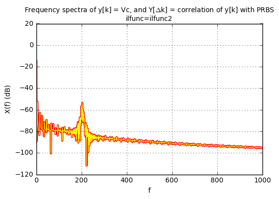
show_freq_spectra(S['Vc'], 'Vc', 'ilfunc=ilfunc1')
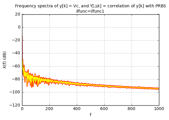
They’re right on top of each other!
So if your original signal without perturbation \( y_0[k] \) has its largest energy in a particular frequency range, so will the correlation \( Y_0[\Delta k] \) between \( y_0[k] \) and an LFSR-based PRBS. (Again, with the caveat that you need to perform the correlation over an entire period of the LFSR.) If I have \( y_0[k] \) with mostly low-frequency content, the power spectral density of the PRBS correlation will be mostly at low-frequencies, and this means that neighboring correlation values don’t change quickly from one value of \( \Delta k \) to the next. If I have \( y_0[k] \) with mostly high-frequency content, so will the PSD of the PRBS correlation \( Y_0[\Delta k] \).
As an example for this high-frequency content, we can use the 202Hz-centered ilfunc2 for the load current \( I_L \):
pn14s = pnr(f14)    # no repeats
kmax = 8192
karray = np.arange(-kmax+1, kmax)
Cc, Ca, S = pn_sysid_nodisturbance(pn14s, karray, ilfunc=ilfunc2)
correlation_waveforms(Cc,[1.0],pn14s,f14,karray,h=None)
crosscorr_title(plt.gca(), pn14s, f14)

show_freq_spectra(S['Vc'], 'Vc', 'ilfunc=ilfunc2')
The signal \( y_0[k] \) is “reflected” into the “PRBS domain” as \( Y_0[\Delta k] \), and if \( y_0[k] \) is unrelated to the PRBS, then its correlation \( Y_0[\Delta k] \) looks like noise. (Reflected pseudonoise!) Whereas if we use the PRBS as an input perturbation, then the corresponding change in output will have a correlation \( Y[\Delta k] \) that looks like the impulse response. The challenge is separating the two, and there isn’t really any way to do so; the only things we can do are to understand and accept the magnitude of the reflected pseudonoise, or increase the magnitude of the perturbation signal so that the signal-to-noise ratio is greater.
Or is there?
Noise Shaping to Enhance PRBS-based System Identification
One thing we can do, if we know something about the spectral density of the background signal \( y_0[k] \), is to try to filter it out. In the frequency spectrum graph of the ilfunc=ilfunc1 case above, most of the energy is in the lower frequencies, whereas the PRBS has energy across the spectrum.
So let’s try applying a high-pass filter to the signal we receive, before computing the correlation.
import scipy.signal

alpha = 0.001
def filter_1pole(y,alpha):
    return scipy.signal.lfilter([alpha], [1,alpha-1], y)
def make_hpf(alpha):
    def f(y):
        y_lpf = filter_1pole(y,alpha)
        return y - y_lpf
    return f
kmax = 500
karray = np.arange(-kmax, kmax)
# no filter
Cc, Ca, S = pn_sysid(pn18,karray)
correlation_waveforms(Cc,Ca,pn18,f18,karray, h_theoretical)

# high pass filter
Cc_hpf, Ca_hpf, S = pn_sysid(pn18,karray,filter=make_hpf(alpha))
correlation_waveforms(Cc_hpf,Ca,pn18,f18,karray, h_theoretical)
Hmm. That really doesn’t help much, except to remove the DC offset.
Getting Those System Parameters, Finally
Now what were we trying to do in the first place? Oh, yeah, estimating these transfer functions:
$$\begin{align} H_A(s) &= \frac{\alpha_A}{1+\tau s} \cr H_B(s) &= \frac{\alpha_B}{1+\tau s} \cr \end{align}$$
with uncertain parameters \( \alpha_A \), \( \alpha_B \), \( \tau \).
A central topic of system identification is devoted to techniques for solving this type of problem, namely determining parameter estimates based on the data we get back from a perturbed system, whether it’s perturbed with sine waves or PRBS.
We’re going to muddle our way through this… again, I’m not an expert in system identification, and the main point of this article is the use of PRBS, which I’ve already shown. But let’s finish this example, by looking at data in a smaller range of \( \Delta k \):
karray = np.arange(0, 32)
pert_ampl = pVa_amplitude
Cc, Ca, S = pn_sysid(pn18,karray,input_amplitude=pert_ampl)
correlation_waveforms(Cc,Ca,pn18,f18,karray, h_theoretical)

This is essentially a nonlinear least-squares problem: we are trying to find constants \( a,b,c \) such that \( C[\Delta k] = ae^{-b\Delta k} + c + n[\Delta k] \) minimizes the mean square error \( n[\Delta k] \). The fact that there doesn’t seem to be much noise in the correlation data is encouraging.
On a PC where we have lots of computing power, estimating those constants is not too hard; scipy.optimize.curve_fit can help, and in fact the example in the documentation is this exact type of function, an exponential with a DC offset. Let’s try it!
import scipy.optimize

def exp_ofs(x, a, b, c):
    return a*np.exp(-b*x) + c

h_measured = Cc/Ca[0]
popt, pcov = scipy.optimize.curve_fit(exp_ofs, karray, h_measured)
a,b,c=popt
print "a=%s, b=%s, c=%s" % (a,b,c)

correlation_waveforms(Cc,Ca,pn18,f18,karray, h_theoretical)
ax = plt.gca()
ax.plot(karray,exp_ofs(karray, a, b, c),'-',linewidth=0.5);
a=0.0866434478506, b=0.0927869720572, c=0.0104562117569

Hurray! We have a really good fit. Now let’s see how close we are to the actual values. First we have to derive the real system values \( \alpha_A \) and \( \tau \) from \( a \) and \( b \):
$$\begin{align} H(s) = \frac{\alpha_A}{1 + \tau s} &\Longleftrightarrow h(t) = \frac{\alpha_A}{\tau}e^{-t/\tau} \cr &\Longleftrightarrow h[\Delta k]=\frac{\alpha_A\Delta t}{\tau}e^{-(\Delta t/\tau)\Delta k} \end{align}$$
so that
$$\begin{align} a &= \alpha_A\Delta t/\tau \cr b &= \Delta t/\tau \cr \tau &= \Delta t/b \cr \alpha_A &= a/b \end{align}$$
Actually, this isn’t 100% accurate; in the equations above, we snuck in a sloppy continous-to-discrete time conversion, and the \( h[\Delta k]=\frac{\alpha_A\Delta t}{\tau}e^{-(\Delta t/\tau)\Delta k} \) equation isn’t exactly correct. If we let \( u=e^{-\Delta t/\tau} \) then for \( \alpha_A=1 \) we should have \( h[\Delta k] = (1-u)\cdot u^k \) so that the sum \( \sum\limits_{k\ge 0} h[\Delta k] = 1 \). (If you don’t remember your z-transform theory, the DC gain of a step response is the step response value as \( t \to \infty \), which is the sum of all the impulse response terms.) So the corrected equation is
$$h[\Delta k]=\alpha_A\left(1-e^{-\Delta t/\tau}\right)e^{-(\Delta t/\tau)\Delta k}$$
which means that
$$\begin{align} a &= \alpha_A\left(1-e^{-\Delta t/\tau}\right)\cr b &= \Delta t/\tau \cr \tau &= \Delta t/b \cr \alpha_A &= a/\left(1-e^{-b}\right) \end{align}$$
import pandas as pd

df_A = pd.DataFrame([dict(estimated = S['dt']/b, actual=S['tau']),
                   dict(estimated = a/(1-np.exp(-b)), actual=S['alpha_A'])],
                  index=['tau','alpha_A'])
df_A| actual | estimated | |
|---|---|---|
| tau | 0.001085 | 0.001078 |
| alpha_A | 0.986486 | 0.977781 |
Now for \( \alpha_B \). This is a little trickier; since the gain is expected to be smaller, we’ll have to bump up the perturbation amplitude in order for the output to be similar. Also, since we expect the same time constant, we can just reuse the one we identified for the A → C channel. This turns things into a linear least-squares problem: \( y = ae^{-bx}+c = au+c \), where \( u=e^{-bx} \), since we’re reusing the exponential constant \( b \). So we can use numpy.linalg.lstsq:
karray = np.arange(0, 32)
pert_ampl = 0.02
Cc, Cb, S = pn_sysid(pn18,karray,input_amplitude=pert_ampl,input_signal='Vb')
def h_theo_b(x):
    return h_theoretical(x,A=alpha_B)
u = np.exp(-b*karray)
A = np.vstack([u,np.ones_like(u)]).T
a, c = np.linalg.lstsq(A,Cc/Cb[0])[0]
correlation_waveforms(Cc,Cb,pn18,f18,karray, h_theo_b)
ax = plt.gca()
ax.plot(karray,a*u+c,'-',linewidth=0.5);
df_B = pd.DataFrame(dict(estimated = a/(1-np.exp(-b)), actual=S['alpha_B']),
                  index=['alpha_B'])
df = pd.concat([df_A,df_B])
df['error (%)'] = (df['estimated'] - df['actual'])/df['actual']*100
df| actual | estimated | error (%) | |
|---|---|---|---|
| tau | 0.001085 | 0.001078 | -0.681724 |
| alpha_A | 0.986486 | 0.977781 | -0.882523 |
| alpha_B | 0.013514 | 0.012825 | -5.092251 |
There! We’re within 1% of the actual values for the results of the “A” experiment, and almost within 5% of actual value for the “B” experiment. We could do better with larger amplitude perturbation. Also, it’s possible to perturb both A and B inputs at the same time, as long as the pseudonoise for each is as uncorrelated as possible; this lets us avoid having to do two separate experiments that take twice the time:
karray = np.arange(0, 32)
def pn_sysid_doitall(karray,pVa,pVb,ilfunc=ilfunc1,seed=1234):
    n = len(pVa)
    assert n == len(pVb)
    S = sysid_sim(Ra=Ra, Rb=Rb, C=C,
                  pVa=pVa,
                  pVb=pVb,
                  N=n,seed=seed,ilfunc=ilfunc)
    # Estimate impulse response as ratio
    # between input and output correlation;
    # we only need input correlation with delay=0
    #
    # Do this for the Va input
    Ca_in      = pncorrelate_array(S['Va'],pVa,[0])
    Ca_out     = pncorrelate_array(S['Vc'],pVa,karray)
    ha_measured = Ca_out/Ca_in[0]

    # And then for the Vb input
    Cb_in      = pncorrelate_array(S['Vb'],pVb,[0])
    Cb_out     = pncorrelate_array(S['Vc'],pVb,karray)
    hb_measured = Cb_out/Cb_in[0]

    # Now estimate tau and alpha_A from the resulting correlation curve
    def exp_ofs(x, a, b, c):
        return a*np.exp(-b*x) + c
    popt, pcov = scipy.optimize.curve_fit(exp_ofs, karray, ha_measured)
    a,b,c=popt
    B = 1-np.exp(-b)
    df_A = pd.DataFrame([dict(estimated = S['dt']/b, actual=S['tau']),
                   dict(estimated = a/B, actual=S['alpha_A'])],
                  index=['tau','alpha_A'])

    # Now estimate alpha_B
    u = np.exp(-b*karray)
    A = np.vstack([u,np.ones_like(u)]).T
    a, c = np.linalg.lstsq(A,hb_measured)[0]
    df_B = pd.DataFrame(dict(estimated = a/B, actual=S['alpha_B']),
                  index=['alpha_B'])

    df = pd.concat([df_A,df_B])
    df['error (%)'] = (df['estimated'] - df['actual'])/df['actual']*100
    return df

pn_sysid_doitall(karray,
                 pVa=0.02*pn18,
pVb=0.1*np.roll(pn18,1000))| actual | estimated | error (%) | |
|---|---|---|---|
| tau | 0.001085 | 0.001083 | -0.173758 |
| alpha_A | 0.986486 | 0.984309 | -0.220742 |
| alpha_B | 0.013514 | 0.013013 | -3.701389 |
The use of pVb=0.1*np.roll(pn18,1000) for the “b” input is a version of the same pseudonoise used for the “A” input, but delayed by 1000 samples. As long as the impulse response of the “A” input doesn’t have any significant content after 1000 samples, this approach is safe to use, and we can use one LFSR to generate both pseudonoise sequences. We don’t actually have to keep a delayed copy of the pseudonoise sequence; if you were paying close attention in Part IX, I mentioned that any delayed version of the LFSR output can be expressed as an XOR of a particular subset of the LFSR state, so we can look for simple XOR combinations of a few of the LFSR state bits and try to find one that has a large delay relative to the normal LFSR output. The libgf2.gf2.GF2TracePattern class can help analyze this:
import libgf2.gf2

trp1 = libgf2.gf2.GF2TracePattern.from_mask(f18,1 << 17)
trp2 = libgf2.gf2.GF2TracePattern.from_mask(f18,1 << 1)
rho = f18.wrap(trp1.pattern) / f18.wrap(trp2.pattern)
n = (1 << f18.degree)-1
print "Expected delay = %d (out of period %d)" % (
    rho.log, n)

bit17 = []
bit1  = []
S = 1
for _ in xrange(n):
    bit17.append((S >> 17) & 1)
    bit1.append((S >> 1) & 1)
    S = f18.mulraw(S, 2)    # shift left
bit17 = np.array(bit17)
bit1  = np.array(bit1)

def bitsof(array, a, b):
    return ''.join('01'[bit] for bit in array[a:b])

print "bit17[0:50]         = %s" % bitsof(bit17,0,50)
print "bit1[0:50]          = %s" % bitsof(bit1,0,50)
d = rho.log
print "bit1[%6d:%6d] = %s" % (d, d+50, bitsof(bit1,d,d+50))
Expected delay = 136155 (out of period 262143) bit17[0:50] = 00000000000000000100000000000010011100000001000001 bit1[0:50] = 01000000000000000011000000000001101001000000110000 bit1[136155:136205] = 00000000000000000100000000000010011100000001000001
Whee! The magic of finite fields helps us again.
Anyway, if we go to really large perturbation amplitudes, we should be able to get the error very low:
pn_sysid_doitall(karray,
                 pVa=10.0*pn18,
pVb=1000.0*np.roll(pn18,1000))| actual | estimated | error (%) | |
|---|---|---|---|
| tau | 0.001085 | 0.001085 | -0.002040 |
| alpha_A | 0.986486 | 0.986485 | -0.000133 |
| alpha_B | 0.013514 | 0.013513 | -0.001995 |
Of course, this is kind of silly; remember, we’re trying to avoid using very large amplitudes. But it does give good evidence that the math is right. (The first time I tried this, I was getting 4-5% error, and finally traced it down to the error in my continuous-to-discrete approximation, hence these lines in sysid_sim():
# match discrete (1-alpha)^n to continuous e^(-dt/tau*n)
alpha = 1-np.exp(-dt/tau)
Normally I gloss over that kind of math, because it’s close enough to just approximate a first-order filter by sticking in \( \alpha \approx \Delta t/\tau \), but when you’re doing system ID and want to be super-accurate, then it’s important to be rigorous.)
Just to make sure we do a little due diligence, let’s look at ilfunc2, the 202Hz-centered load current:
pn_sysid_doitall(karray,
                 pVa=0.02*pn18,
                 pVb=0.1*np.roll(pn18,1000),
ilfunc=ilfunc2)| actual | estimated | error (%) | |
|---|---|---|---|
| tau | 0.001085 | 0.001067 | -1.686920 |
| alpha_A | 0.986486 | 0.965136 | -2.164296 |
| alpha_B | 0.013514 | 0.014722 | 8.945755 |
It’s the same order-of-magnitude error.
Error analysis
We can be a little more rigorous by repeating it 10 times with different random seeds, and seeing how the statistics work out:
from IPython.display import display

def error_analysis(rel_magn_list, npoints, ilfunc, pn, vbdelay=1000):
    for relative_magn in rel_magn_list:
        print "relative magnitude rho =", relative_magn
        print "normalized errors (rho * % error of actual value) :"
        errors = []
        for seed in (np.arange(npoints) + 1234):
            df=pn_sysid_doitall(karray,
                         pVa=relative_magn*0.02*pn,
                         pVb=relative_magn*0.1*np.roll(pn,vbdelay),
                         ilfunc=ilfunc,
                         seed=seed)
            errors.append(df['error (%)'])
        norm_errors = pd.DataFrame(errors) * relative_magn
        norm_error_stats = pd.DataFrame(dict(mean=norm_errors.mean(),
                                        std=norm_errors.std()))
        display(norm_error_stats)

error_analysis(rel_magn_list=[0.25, 1, 4.0], npoints=10,
               pn=pn18, ilfunc=ilfunc1)
relative magnitude rho = 0.25 normalized errors (rho * % error of actual value) :
| mean | std | |
|---|---|---|
| tau | -0.289310 | 0.478065 |
| alpha_A | -0.009466 | 0.686041 |
| alpha_B | -1.124795 | 2.933403 |
relative magnitude rho = 1 normalized errors (rho * % error of actual value) :
| mean | std | |
|---|---|---|
| tau | -0.300446 | 0.489609 |
| alpha_A | -0.019726 | 0.698977 |
| alpha_B | -1.128359 | 2.915813 |
relative magnitude rho = 4.0 normalized errors (rho * % error of actual value) :
| mean | std | |
|---|---|---|
| tau | -0.31693 | 0.492590 |
| alpha_A | -0.02189 | 0.702373 |
| alpha_B | -1.12419 | 2.911618 |
The errors are essentially inversely proportional to the perturbation amplitude: if we increase the perturbation amplitude by a factor of 4, then we decrease the error by a factor of 4; if we decrease the perturbation amplitude by a factor of 4, then we increase the error by a factor of 4.
Here’s the same kind of experiment for the 202Hz load current, ilfunc2:
error_analysis(rel_magn_list=[0.25, 1, 4.0], npoints=10, pn=pn18, ilfunc=ilfunc2)
relative magnitude rho = 0.25
normalized errors (rho * % error of actual value) :
| mean | std | |
|---|---|---|
| tau | -0.339801 | 2.809975 |
| alpha_A | 0.075691 | 4.273403 |
| alpha_B | 9.510804 | 25.856302 |
relative magnitude rho = 1
normalized errors (rho * % error of actual value) :
| mean | std | |
|---|---|---|
| tau | -0.478069 | 2.739761 |
| alpha_A | -0.206227 | 3.995722 |
| alpha_B | 8.939591 | 25.211266 |
relative magnitude rho = 4.0
normalized errors (rho * % error of actual value) :
| mean | std | |
|---|---|---|
| tau | -0.526279 | 2.726861 |
| alpha_A | -0.273868 | 3.946693 |
| alpha_B | 8.806005 | 25.104261 |
The numbers are different (we get a larger error for ilfunc2) but the behavior is the same: increase the signal amplitude by a factor of K, and the error goes down by a factor of K.
Why are the estimation errors larger for ilfunc2? Because it has most of its energy at higher frequencies, and this means the PSD of reflected pseudonoise (when we correlate the system with pseudonoise) also has its content at higher frequencies. Whereas the current in ilfunc1, even though it has about the same amplitude, has most of its energy at low frequencies, and this means the PSD of reflected pseudonoise has most of its content at low frequencies.
So what? Well, we’re using a parameter estimation technique to estimate \( a, b, c \) of \( h[\Delta k] = ae^{-b\Delta k}+c \), which does a very good job of disregarding the DC offset \( c \), and because we’re working over a small number of samples of the impulse response (32 out of 262143 in the examples in this article), only the high-frequency content of the reflected pseudonoise contributes significantly towards estimation error; the low-frequency content of the reflected pseudonoise looks like DC, and we can remove it as an unknown DC offset. So ilfunc1‘s reflected pseudonoise gets rejected for the most part, whereas ilfunc2 does not.
What this means is that if you’re working with systems that have most of their frequency content at frequencies much lower than the Nyquist frequency (half the sampling frequency), then the technique given in this article should work reasonably well. Whereas if there’s lots of content at higher frequencies then it’s not so good.
Now let’s look at the effect on the estimated parameters if we change the number of samples.
Here’s the same kind of thing with ilfunc1 using one cycle of a 16-bit LFSR. I would expect that the errors are twice as bad as an 18-bit LFSR, since our error for \( n \) samples should be proportional to \( 1/\sqrt{n} \). For four cycles of a 16-bit LFSR I would expect similar performance as one cycle of an 18-bit LFSR.
print "One cycle of %s:" % f16
pn16 = pnr(f16, 16)
error_analysis(rel_magn_list=[0.25, 1, 4.0], npoints=10,
pn=pn16, ilfunc=ilfunc1)
print "Four cycles of %s:" %f16
pn16 = pnr(f16, 18)
error_analysis(rel_magn_list=[0.25, 1, 4.0], npoints=10,
pn=pn16, ilfunc=ilfunc1)One cycle of GF2QuotientRing(0b10000000000101101): relative magnitude rho = 0.25 normalized errors (rho * % error of actual value) :
| mean | std | |
|---|---|---|
| tau | -0.243775 | 0.492968 |
| alpha_A | 1.254509 | 0.969835 |
| alpha_B | 4.497856 | 3.539538 |
relative magnitude rho = 1
normalized errors (rho * % error of actual value) :
| mean | std | |
|---|---|---|
| tau | -0.260740 | 0.510994 |
| alpha_A | 1.260187 | 0.973230 |
| alpha_B | 4.849147 | 3.734219 |
relative magnitude rho = 4.0
normalized errors (rho * % error of actual value) :
| mean | std | |
|---|---|---|
| tau | -0.296083 | 0.515723 |
| alpha_A | 1.304284 | 0.974139 |
| alpha_B | 5.606268 | 3.786611 |
Four cycles of GF2QuotientRing(0b10000000000101101): relative magnitude rho = 0.25 normalized errors (rho * % error of actual value) :
| mean | std | |
|---|---|---|
| tau | 0.016211 | 0.400911 |
| alpha_A | 0.366903 | 0.612219 |
| alpha_B | 0.368435 | 2.488373 |
relative magnitude rho = 1
normalized errors (rho * % error of actual value) :
| mean | std | |
|---|---|---|
| tau | 0.012102 | 0.404466 |
| alpha_A | 0.364922 | 0.612005 |
| alpha_B | 0.425626 | 2.474830 |
relative magnitude rho = 4.0
normalized errors (rho * % error of actual value) :
| mean | std | |
|---|---|---|
| tau | 0.003310 | 0.405377 |
| alpha_A | 0.378318 | 0.611995 |
| alpha_B | 0.609967 | 2.471524 |
Hmm. It’s not clear what’s going on here. We saw earlier that the reflected pseudonoise definitely has that \( 1/\sqrt{n} \) behavior, but how that impacts the parameter estimation is not really clear, and it looks like there are some nonlinearities, because the mean value of the error is not zero. (Which technically means that the estimation technique I used was not an unbiased estimator, and we should be able to do better… but my brain is really starting to hurt here, so I’ll just let it go.)
What About Second-Order Systems? Closed-loop Systems?
We looked at a first-order system. What about a second-order system? I’m going to leave that exploration to the reader; the only difference is that you’d need to analyze the impulse response to estimate the poles and DC gain. This isn’t trivial, especially if the system behavior has wide dynamic range and the poles are very far apart. For example, even a 2nd-order system with a pole at 1Hz and the other at 1000Hz presents problems, since the transfer function amplitude at the 1000Hz pole is 1000 times smaller than at the 1Hz pole — the behavior at the higher-frequency pole is very hard to pick up.
Closed-loop systems are a challenge as well; if you perturb the system, the controller will tend to try to cancel out that perturbation. So it can be difficult in some frequency ranges to apply a perturbation signal under closed-loop control.
What About Embedded Systems?
Some of these calculations are feasible to implement on resource-limited embedded systems, and others aren’t. Here’s my take on it:
- LFSR pseudonoise generation: yes
- Computation of correlation: yes (for a limited number of samples of the impulse response, like 16 or 32; all we’re really doing is either adding or subtracting from an accumulator, depending on whether the pseudonoise bit is 1 or 0.)
- Estimation of parameters: tricky – nonlinear least squares is probably not feasible, but some kind of simplified recursive-least squares analysis is probably doable, especially if the uncertain parameters are known to lie within a narrow band, for example, 1 millisecond ± 10%. (Watch out though; recursive algorithms can have stability issues.) Or the clever engineer might be able to think of a simpler algorithm that is not as accurate but requires less computation.
I’d even note that the LFSR pseudonoise and correlation computations can be done by a low-end 8-bit processor! All that’s necessary are bit shifts, XORs, addition, and subtraction, although the variables containing accumulated cross-correlation signals may need to be extended to 16- or 32-bit values to avoid overflow.
Wrapup
Whew! We covered quite a bit of ground on the topic of system identification using a pseudorandom bit sequence (PRBS) from an LFSR. (And yet, as far as system identification goes, this is just scratching the surface!)
-
System identification attempts to estimate uncertain or unknown parameters by observing system inputs and outputs.
-
In many cases the observed signals can be enhanced by perturbing some of those inputs.
-
Sine-wave perturbations can be used to estimate frequency-domain response, by correlating system inputs and outputs, one frequency at a time.
-
PRBS from an LFSR can be used as a perturbation signal to estimate impulse response in the time domain, by correlating system inputs and outputs. This works because the cross-correlation between the PRBS and a time-shifted version of the same sequence is nearly zero, forming a quasi-orthonormal basis.
-
The amplitudes of the frequency spectra of the following two signals are the same (except at DC):
- Any waveform \( y[k] \)
- The cross-correlation of \( y[k] \) with a PRBS over an integer number of periods
-
The cross-correlation of the system output with a PRBS perturbation has two parts:
- “Reflected pseudonoise” — this is the cross-correlation between PRBS and the “normal” system output (without perturbation)
- Impulse response cross-correlation — this represents cross-correlation between PRBS and the system output’s response to that perturbation, and it approximates the impulse response of the system transfer function
-
The amplitude of “reflected pseudonoise” is proportional (relative to the impulse response cross-correlation) to \( 1/\sqrt{n} \) where \( n \) is the number of samples.
-
Parameter estimation of a first-order system from the impulse response cross-correlation can be computed using nonlinear least squares.
-
Increasing the amplitude of the PRBS perturbation by a factor of \( K \) increases the impulse response cross-correlation by the same factor \( K \), and decreases the relative error of estimated parameters by approximately the same factor \( K \)
One more time: I’m not an expert in the field of system identification, so if one of you reads this article and finds some silly mistakes or inaccurate statements, please let me know about them, so I can improve it.
References
Unfortunately I have not found any really good references for this application of linear-feedback shift registers. The “classic” in the field of system identification is Ljung:
- Lennart Ljung, System Identification: Theory for the User, Prentice-Hall, 2nd edition, 1999.
Not only is this literally the book that the MATLAB System Identification Toolbox is based on, but Professor Ljung was the primary author of this toolbox. I don’t find it very readable at all; perhaps if you are a graduate student in control theory and estimation you will gobble up this material like you would a bowl full of potato chips, but I find it very impenetrable. Here’s an example:
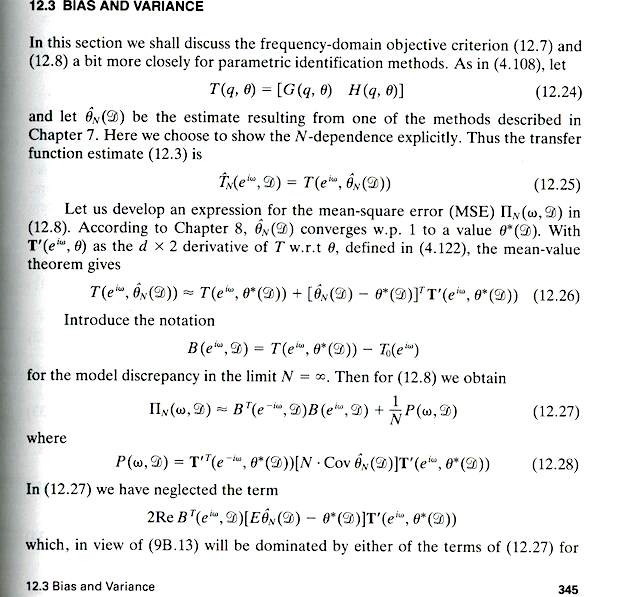
Also, it has an awful name; the word “user” is primarily applied to drug addicts and customers of computer software, neither of which applies here. I bought a used copy, and the one saving grace that prevented me from angrily chucking the thing at the trash can — besides the fact that I did spend money on it — was Chapter 14, “Experiment Design”, which does have some useful practical advice, if you can get past all the \( \operatorname{arg} \operatorname{min} \) equations and those arcane cursive math fonts like \( \mathscr{ H D } \) to represent some abstract universe of things. (\( \mathscr{ D } \) = {all design variables A to D}, according to p. 340, following a long list of implementation choices with sections A - D.) Chapter 14 goes into topics like pretreatment of data with filtering, or choice of sampling interval. Unfortunately it’s a very short chapter.
Sigh. But maybe you’ll get something valuable out of reading Ljung.
Let me know if you find any other good references on the topic!
Next time we’ll cover one of the communications applications of LFSRs, namely Gold codes. And I promise it will be a much shorter article.
© 2018 Jason M. Sachs, all rights reserved.


- Comments
- Write a Comment Select to add a comment
The practical application of this is described in "
TMS320f28069-Based Impedance Spectroscopy With Binary
Excitation" by Rist, Reidla, Min, Parve, Martens and Land.
It might be under patent though.
To post reply to a comment, click on the 'reply' button attached to each comment. To post a new comment (not a reply to a comment) check out the 'Write a Comment' tab at the top of the comments.
Please login (on the right) if you already have an account on this platform.
Otherwise, please use this form to register (free) an join one of the largest online community for Electrical/Embedded/DSP/FPGA/ML engineers:


