Linear Feedback Shift Registers for the Uninitiated, Part XIV: Gold Codes

Jason Sachs●April 18, 2018

Last time we looked at some techniques using LFSR output for system identification, making use of the peculiar autocorrelation properties of pseudorandom bit sequences (PRBS) derived from an LFSR.

This time we’re going to jump back to the field of communications, to look at an invention called Gold codes and why a single maximum-length PRBS isn’t enough to save the world using spread-spectrum technology. We have to cover two little side discussions before we can get into Gold codes, though.

(I will have to add another disclaimer here, that I am not an expert in communications theory… it’s possible that I goofed in my reasoning somewhere, so if you read this and see an example that just makes no sense, please let me know, so I can fix the error.)

Spread-spectrum: A Recap

First of all, I realized that in all of my talk about spread-spectrum systems in part XII, not once did I show a block diagram of one. We’ll have to fix that. Here’s a direct-sequence spread-spectrum (DSSS) block diagram:

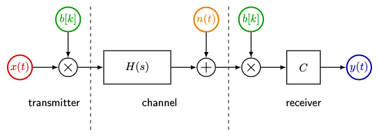
From left to right, we have:

a transmitter, which includes
- some important input $ x(t) $, the message we are trying to transmit
- a PRBS $ b[k] $ which takes on values $ \pm 1 $
- we modulate $ x(t) $ with $ b[k] $ (multiplying the two together) and transmit
a channel, which contains
- some kind of transfer function $ H(s) $, typically a combination of delay, attenuation, and filtering
- noise, modeled here as additive noise $ n(t) $
a receiver, which includes
- a PRBS $ b[k] $
- a demodulator, where we multiply by $ b[k] $ in the hopes of canceling out the multiplication on the transmitter side
- a correlator $ C $
- output $ y(t) $

The goal is to reconstruct $ y(t) \approx x(t - T_1) $ from $ x(t) $, where $ T_1 $ is some transmission and processing delay. We gloss over a few important details:

radiofrequency modulation is not shown — typically the modulated output of the transmitter is only an intermediate frequency (IF) output, that is itself modulated on some sinusoidal carrier frequency. If we use a 10MHz chip rate for $ b[k] $ then the IF output covers 0-10MHz, and we need to shift that band upwards to whatever range of carrier frequencies at which we are trying to transmit. Then we can choose the spread-spectrum bandwidth and the center frequency independently. Otherwise it is truly a direct-sequence spread-spectrum transmitter, and two things are going to occur:
- if we’re using wireless transmission, the low-frequency content is not going to transmit well
- the chip rate is coupled to the frequency range we want to cover.
radiofrequency demodulation is not shown — same issue at the receiver
synchronization — how the heck do we reconstruct the PRBS $ b[k] $ properly in the receiver?
correlation — what is the $ C $ block doing? In part XII we used an integrate-and-dump receiver that integrates the received and demodulated samples, and then outputs a 1 if the integrator is positive, 0 if it’s not… and then at the end of each chip, the integrator is reset. There are other ways of doing this — look up Bayesian receivers and rake receivers; I’m just as lost as you are.

Synchronization and correlation are some really hard problems, and I have no idea what kind of magic techniques are used in the communication industry. Every couple of years I get inspired to try to get up to speed with LFSR synchronization techniques, and I just fail.

But that’s not what these articles are about, we’re just trying to show the basic ideas of spread-spectrum, particularly around the PRBS itself.

Schrödinger’s Highway: Let’s Talk About Traffic Flow

The second little diversion has to do with the fact that today’s article is going to touch on a very subtle aspect of spread-spectrum theory — what happens when you operate asynchronously — and why Gold codes work the way they do. (It seems subtle to me, at least.) So before we jump back in, we’re going to have a brief little thought experiment.

Picture this:

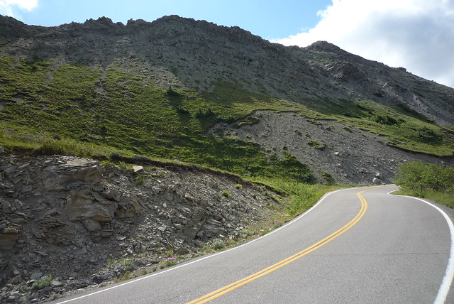
You are driving your fantasy car, somewhere on a highway in the western United States. Maybe it’s a Mustang convertible, or a VW Westphalia, or a classic 1950’s Studebaker, or a Tesla Model 3. Whatever. Get in your happy place.

It’s a sunny day, not too hot, and you’re all alone with miles of scenery, driving at some speed $ v $. You are in zen mode, just you and the road and nothing else. Turn the radio up loud!

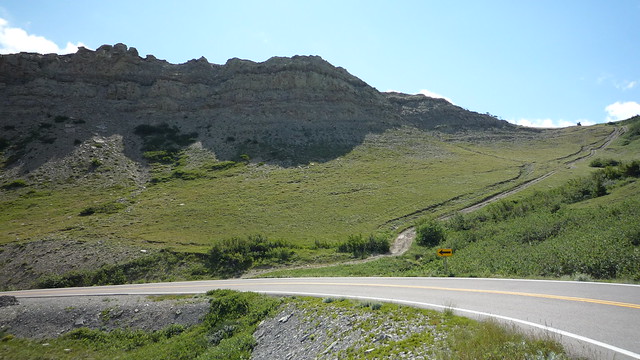
Now all of a sudden you see traffic ahead. You cannot maintain speed $ v $ anymore; you will have to slow down to some lower speed to avoid hitting the car in front of you. It’s not awful traffic, and you’re still going at a decent speed… let’s say it’s $ 0.95v $. That’s 95% of what speed you’d be traveling if there weren’t all these other beastly cars on the road. Because now you’re no longer letting your mind roam free while listening to your favorite music. Instead, you’ve got to pay attention to all these other cars and adjust your acceleration and braking accordingly. You cannot choose a speed; instead, you have to travel more or less the same speed as the other cars. All this to avoid hitting someone.

Here’s a question: how dense is the traffic?

In other words, when the road starts to get just a bit congested, what percentage of the road surface is covered by cars? Take a guess!

It turns out that the widthwise density on US interstate highways is about 50%, and for a speed of 114km/hr (70.8mph), the lengthwise density just prior to congestion is about 6%, for a net coverage of only 3%, not including the road shoulders, which would make it even lower.

Now here’s the fun part:

Imagine we had a magic switch, that could spread out the atoms of our car by a factor of 512, and instead of hitting another car, we would just kind of pass through with a warm-and-fuzzy feeling. Sort of a superposition of Studebakers. We could, in fact, have three cars in the same location. Or even four cars. At some point it would stop being warm and fuzzy, but let’s say that we could get to the same area density as “conventional” traffic, or 1/32, before we got to a risk of injury. With a spreading of 512, we could put 16 cars in the same position before reaching that point.

The highways have the same capacity — we no longer need that distance between cars to keep them safe; instead we need to keep the atomic density down — but now there’s no speed restriction. I can go at 120km/hr, someone else can go at 122km/hr, another person can drive at 119km/hr. No need to worry about where the edge of the car is. No more idiots and maniacs. My stress level would go way down.

Back from Fantasyland

The point of that weird little thought experiment has to do with the relation between the spread-spectrum technique in Part XII and the use of Gold codes.

In Part XII I showed this wonderful example of two spread-spectrum transmitters that used the same PRBS, but shifted to different positions. No problem! It’s almost a perfect example of uncorrelated transmitters, as long as they don’t overlap in phase. If two transmitters are both sending with the same phase of PRBS, then BOOM, there’s a collision, and we have a likely communications error.

You might think, well, that’s not too hard to avoid, we’ll all just maintain a safe distance in phase from each other. But there are a few problems here.

One is that this requires some sort of mutual synchronization. Let’s suppose for a moment that the transmitters don’t have to be synchronized in frequency. If I’ve got a transmitter cycling through the PRBS at 10MHz and you’re cycling through the same PRBS at 10.02MHz, then we’re going to experience a beat frequency of 20kHz: every 50 microseconds, the bit edges are going to line up, then shift apart, then line up again. If we have a PRBS with a period of, say, 1023, then every 51.1 milliseconds (50 μs × 1023) we’re going to have a short time, maybe 50 microseconds, in which the PRBS phases are aligned and the signals interfere with each other. To avoid this problem, we need to either make sure we all transmit at the same frequency and stay separated in phase — just like cars in congested traffic stay separated in distance on the highway but generally travel at the same speed — or tolerate the consequences of periodic phase alignment and interference. In other words, asynchronous operation at approximately the same frequency causes worst-case synchronous behavior from time to time.

The other problems involve the effect of increasing the number of transmitters that share “space” with each other, and the effect of physical separation on phases at the receiver. These problems essentially ruin a system where all transmitters share a single common PRBS; we’ll go into some detail later on in this article.

Gold codes solve this problem by constructing a set of multiple PRBS, where the worst-case correlation between any two pairs of sequences is bounded to a small number. Not as small as the cross-correlation between transmitters of the same PRBS at different phases, but unlike this case, no matter what the phase alignment of a pair of PRBS, there is no way to achieve high correlation. They do this trading off worst-case and best-case correlation, much like our Schrödinger’s highway, where the cars don’t collide, instead they just pass through each other with a warm and fuzzy feeling.

If we have a common 15-bit maximum-length PRBS with period 32767, for example, the correlation function is either -1 for misaligned phases or 32767 for aligned phases. With two separate Gold codes of period 32767, the maximum amplitude of the correlation function is 257, no matter what the relative phase is.

That’s kind of handwavy, and to explain it better, we need some more details. Time for some mathematics and Python.

Looking Again at a Common PRBS

Now, in the previous two parts in this series, we looked at basic spread-spectrum techniques which rely on the fact that the autocorrelation function $ R_{bb}[\Delta k] $ (or normalized correlation $ C_{bb}[\Delta k] $) of a particular class of PRBS $ b[k] $ is two-valued:

$$\begin{align} R_{bb}[\Delta k] &= \sum\limits_{k=0}^{n-1} b[k]b[k-\Delta k] = \begin{cases} n & \Delta k = 0 \cr -1 & \Delta k \ne 0 \end{cases} \cr C_{bb}[\Delta k] &= \tfrac{1}{n}\sum\limits_{k=0}^{n-1} b[k]b[k-\Delta k] = \begin{cases} 1 & \Delta k = 0 \cr -\frac{1}{n} & \Delta k \ne 0 \end{cases} \end{align}$$

We’re going to be using the correlation function bunch of times, but before we do, I’m going to get impatient if we don’t use a fast algorithm for computing correlation using the FFT, which we alluded to in part XIII, namely the fact that the Fourier transform of the correlation is the conjugate product of the Fourier transforms of its inputs:

$$\mathcal{F}(R _ {xy}[\Delta k]) = \mathcal{F}(x)\overline{\mathcal{F}(y)}$$

where $ \overline{z} $ denotes the conjugate of some value $ z $. Restated another way, we can get the cross-correlation as follows:

$$R _ {xy}[\Delta k] = \mathcal{F}^{-1}(\mathcal{F}(x)\overline{\mathcal{F}(y)})$$

This can really speed up computation, at the cost of some accuracy....

import numpy as np
from libgf2.gf2 import GF2QuotientRing, checkPeriod

def lfsr_output(field, initial_state=1, nbits=None, delay=0):
    N = field.degree
    if nbits is None:
        nbits = (1 << N) - 1
    u = field.rshiftraw(initial_state,delay)
    for _ in xrange(nbits):
        yield (u >> (N-1)) & 1
        u = field.lshiftraw1(u)

def pnr_base(field, nbits, delay):
    return np.array(list(
            lfsr_output(field, nbits=nbits, delay=delay))) * 2 - 1
        
def pnr_unopt(field, N=None, nbits=None, delay=0):
    """ pseudonoise, repeated to approx 2^N samples 
    (unoptimized)
    """
    N0 = field.degree
    period = (1<<N0) - 1
    if nbits is None:
        if N is None:
            N = N0
        nbits = period * (1<<(N-N0))
    return pnr_base(field, nbits, delay)
        
def pnr(field, N=None, nbits=None, delay=0):
    """ pseudonoise, repeated to approx 2^N samples """
    N0 = field.degree
    period = (1<<N0) - 1
    if nbits is None:
        if N is None:
            N = N0
        nbits = period * (1<<(N-N0))
    if nbits <= period:
        return pnr_base(field, nbits, delay)
    b = pnr_base(field, period, delay)
    nrepeat = (nbits + (period-1)) // period
    return np.tile(b, nrepeat)[:nbits]
        
def circ_correlation(x, y):
    """circular cross-correlation"""
    assert len(x) == len(y)
    return np.correlate(x, np.hstack((y[1:], y)), mode='valid')

def circ_correlation_fft(x,y,result_type=float):
    """circular cross-correlation using fft"""
    assert len(x) == len(y)
    result = np.fft.ifft(np.fft.fft(x) * np.conj(np.fft.fft(y)))
    if result_type==float:
        result = np.real(result)
    if result_type==int:
        result = np.round(np.real(result)).astype(int)
    # we really should raise an error if the result isn't close
    # to a real number or an integer, not just throw away info
    return result

import time 

f14 = GF2QuotientRing(0x402b)
p14 = (1<<14) - 1
assert checkPeriod(f14,p14) == p14
pn14 = pnr(f14)

f15 = GF2QuotientRing(0x8003)
p15 = (1<<15) - 1
assert checkPeriod(f15,p15) == p15
pn15 = pnr(f15)

f16 = GF2QuotientRing(0x1002d)
p16 = (1<<16) - 1
assert checkPeriod(f16,p16) == p16
pn16 = pnr(f16)

def compare_correlation(x,y):
    t0 = time.time()
    a = circ_correlation(x, y)
    t1 = time.time()
    b = circ_correlation_fft(x, y)
    t2 = time.time()
    return a,b,t1-t0,t2-t1

for pn,N in ((pn14,14), (pn15,15), (pn16,16)):
    a,b,ta,tb=compare_correlation(pn,pn)
    print "%d-bit LFSR (%d samples):" % (N,len(pn))
    print "time of circ_correlation:     %.3fs" % ta
    print "time of circ_correlation_fft: %.3fs" % tb
    print "max error in difference:      %g" % np.max(np.abs(b-a))
    print "a[0] = %s, b[0] = %.14f" % (a[0],b[0])
    print ""

print "for pn16:"
b2 = circ_correlation_fft(pn16,pn16,result_type=int)
assert (b2[1:] == -1).all()
print "b2 =", b2

14-bit LFSR (16383 samples):
time of circ_correlation:     0.279s
time of circ_correlation_fft: 0.015s
max error in difference:      1.02893e-11
a[0] = 16383, b[0] = 16383.00000000000182

15-bit LFSR (32767 samples):
time of circ_correlation:     1.110s
time of circ_correlation_fft: 0.036s
max error in difference:      2.23401e-11
a[0] = 32767, b[0] = 32767.00000000000000

16-bit LFSR (65535 samples):
time of circ_correlation:     4.476s
time of circ_correlation_fft: 0.097s
max error in difference:      4.14679e-11
a[0] = 65535, b[0] = 65535.00000000000728

for pn16:
b2 = [65535    -1    -1 ...,    -1    -1    -1]

Note that the FFT-based computation of correlation is much quicker, by a factor of 50 for a period of 65535. Doubling the length essentially quadruples the time to calculate using np.correlate — it’s actually $ O(n^2) $ — but only increases the time using FFT-based calculations by a little more than double — it’s actually $ O(n \log n) $.

OK, now back to the math. The reason we want this particular two-valued autocorrelation is that it means that the PRBS is almost an orthonormal basis. It would be a perfect orthonormal basis if the autocorrelation function were zero for delays other than zero. Even if it’s not perfectly orthonormal, if we have a very small correlation for shifted versions of the PRBS, this means that the signals can easily be distinguished from each other. Effectively there’s a gain of $ n $ (where $ n $ is the length of the sequence) for the PRBS with no shift, and a gain of $ -1 $ for shifted versions of the PRBS, and this lets us selectively recover the original PRBS with its modulation amplitude $ x(t) $ — assuming $ x(t) $ changes much more slowly than the chip rate — and discard delayed versions.

Suppose I have two transmitters producing spread-spectrum sequences $ y_1[k] $ and $ y_2[k] $. If they use the same PRBS but shifted from each other, then the correlation between these sequences is almost zero, and we can recover those sequences very easily without interference. We saw this in part XII, in which I mentioned:

There is a catch here; we have to keep the chipping sequences uncorrelated. One way to do this is use the same LFSR output sequence, shifted in time — as we did in this contrived example — but that’s not really practical, because it would require time synchronization among all transmitters. Without such time synchronization, there’s a small chance that two transmitters would use a chipping sequence which is close enough that they would interfere, and the birthday paradox says that this goes up as the square of the number of transmitters.

So if we have a 16-bit LFSR shared among two transmitters, without trying to synchronize them in time, then there’s a one-in-65535 chance that the chipping sequences will overlap, and we’ll have interference due to their high correlation. If we have three transmitters, then the chance of interference among any pair is $ 1 - \frac{65534}{65535}\cdot\frac{65533}{65535} \approx \frac{3}{65535} $. If we have four transmitters, it goes up to approximately $ \frac{6}{65535} $, and with five transmitters it goes up to approximately $ \frac{10}{65535} $.

OK, you might say, big deal; if you crunch the math then it takes 117 transmitters before there is more than a 10% chance of interference between any pair of transmitters:

# p = probability of no interference
p = 1
n_transmitters = 117
for k in xrange(1,n_transmitters+1):
    p *= (65535-k)/65535.0
1-p

0.10003196810651538

And even then we could just detect interference and try to use a different shift value for the PRBS, right?

Well… that would be nice… but here are some problems with communications that make the situation even worse.

Path delay

Transmitters and receivers are located at different positions — that’s why we’re trying to communicate! This means that the time delay between received signals depends on the location of the receiver. Let’s say we’re using a 10MHz chipping sequence, so each bit of the PRBS lasts 100ns. The speed of electromagnetic radiation (whether it’s light, or 900MHz radio) is approximately 3 × 10⁸ m/s = 30cm per nanosecond in air or vacuum, and that means that if we’re transmitting wireless signals, they travel 30 meters in 100ns.

Why does that matter? This is one of those cases where a picture is worth a thousand words. Suppose we have transmitters A and B that are 90m apart, or 3 chips. B is 90m north of A, and the time it takes for a signal to get from point A to point B (or vice versa) is the same time it takes to transmit 3 bits of the PRBS.

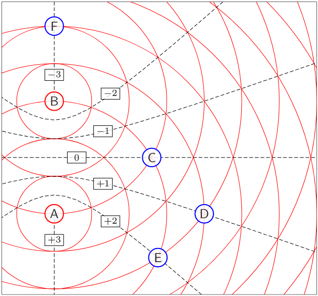
Each of the thin red circles in this diagram represents an additional distance of 30m, or 1 chip, and they spread out like ripples in a pond.

Now let’s look at some receivers:

Receiver C is 90m from both A and B. Signals take the same time to get from A and B.
Receiver D is 120m from A, and 150m from B. This means that signals take 30m, or 1 chip, longer to get from B to D, than from A to D. So effectively, as far as D sees, the signal from A is shifted ahead by +1 chip, relative to the signal from B.
Receiver E is 90m from A, and 150m from B. So effectively the signal from A is shifted by +2 chips, relative to the signal from B.
Receiver F is 60m from B, and 150m from A. So effectively the signal from A is shifted by -3 chips, relative to the signal from B.

The dotted lines show points of constant relative delay, and are hyperbolic curves of the following form:

$$ \frac{4y^2}{D^2} - \frac{4x^2}{d^2 - D^2} = 1$$

where $ d $ is the distance between transmitters, $ D = c\Delta t $ is the relative distance seen by a receiver, $ c $ is the speed of wave propagation, and $ \Delta t $ is the relative time shift seen by a receiver.

Now, if we’re using the same PRBS (but shifted) for spread-spectrum for both transmitters A and B, then any relative shift of the PRBS between $ -3 $ and $ +3 $ chips is no good, because there will be a receiver anywhere along one of those particular hyperbolic curves where the relative shifts are zero, and then the two PRBS are correlated, so we have no way of distinguishing received messages $ x_A(t) $ from $ x_B(t) $. They both are modulating the PRBS in a way that synchronized with identical phase at the receiver.

If A and B use the same PRBS, with a relative shift of more than 4 chips, then we won’t have a problem. This effectively reduces the number of transmitters that can share the same PRBS without interference, by a factor that relates to the distance between transmitters.

With transmitters and receivers that are in close proximity — the propagation delay from transmitter to receiver is significantly smaller than the time of one PRBS chip, or 30m in this particular case — this isn’t a problem, but for large distances it effectively kills the use of spread-spectrum using a common PRBS with different shifts, greatly reducing the number of different shift values that can be used to discriminate among multiple transceivers.

Multipath delays

In open space, it’s easy to define the time it takes a signal to arrive from, say, transmitter A to receiver D. In the real world, there are walls and windows and things that can cause reflections. This means that part of the signal from A to D that travels directly takes 400ns to arrive, but if there’s a metal garage door nearby, then another part of the signal that bounces off the garage door takes 500ns to arrive.

This effectively increases the different locations that would cause interference, if a common PRBS is used.

What’s a transmitter to do?

OK, so in practice, other techniques are used. We could for example, have transmitter A use an LFSR with one polynomial, and transmitter B use an LFSR with a different polynomial. Let’s try it and look at the maximum correlation between LFSR outputs of various 15-bit polynomials. We’ll look at how the first polynomial compares with all of the remaining polynomials:

# let's use 15-bit polynomials... why? just because
fields = []
maxcount = 10000
for k in xrange(2,32768,2):
    poly = p15 + k
    if checkPeriod(poly,p15) == p15:
        fields.append(GF2QuotientRing(poly))
        if len(fields) >= maxcount:
            break

pn15_0 = pnr(fields[0])
Rmax = {}

for f in fields[1:]:
    pn15_other = pnr(f)
    R = circ_correlation_fft(pn15_0, pn15_other, result_type=int)
    Rmax[f.coeffs] = np.abs(R).max()

import pandas as pd

pd.set_option('display.max_rows', 20)

Rmaxs = pd.Series(Rmax)
V = Rmaxs.value_counts()
V.sort_index(inplace=True)
V = pd.DataFrame(V,columns=["count"])
V.index.name = "correlation"
V

	count
correlation
257	18
361	1
513	42
545	2
575	12
577	76
585	2
591	2
607	6
609	16
...	...
1695	2
1727	2
1887	2
2047	6
2113	2
2175	2
2495	2
4799	2
4863	1
4927	2

84 rows × 1 columns

Remember, perfect correlation would give us a result of $ n=32767 $. The maximum correlations range from a minimum of 257 ($ \approx 0.0078n $) to a maximum of 4927 ($ \approx 0.15n $).

There were 18 polynomials that allowed us to achieve the minimum (257) worst-case correlation. Is there anything special about these polynomials?

The Three-Valued Cross-Correlation Theorem

It turns out that there is, at least for some of the polynomials. Perhaps you remember from part IX that there is a way to determine the decimation ratio between quotient rings: that is, if we take a maximum-length output sequence $ b_1[k] $ derived from some quotient ring $ GF(2)[x]/p_1(x) $ and decimate by some integer $ j $, taking every $ j $th value, we’ll get another maximum-length output sequence $ b_2[k] = b_1[jk] $ derived from a different quotient ring $ GF(2)[x]/p_j(x) $. If we have the bit sequences, we can go from there to the polynomials $ p_1(x) $ and $ p_j(x) $ using the Berlekamp-Massey algorithm; once we have these polynomials, we can do some fancy stuff with finite fields to determine the decimation ratio $ j $, although we can’t distinguish decimation by $ j $, $ 2j $, $ 4j $, etc.

My Python module libgf2, which no one else actually uses, contains a routine called libgf2.lfsr.undecimate which will compute the value of $ j $:

min_corr_poly_list = sorted([p for p in Rmax if Rmax[p] == 257])
print '\n'.join('%x' % p for p in min_corr_poly_list)

80cf
8423
8729
8785
900b
9211
9a5d
b2ef
be37
c631
d4d3
d9f9
ed97
edab
facb
fae5
fb0f
fc75

from libgf2.lfsr import undecimate, decimate

# field and pseudonoise of first field (0x8003)
qr0 = fields[0]
pn0 = pnr(qr0)
decimation_ratios = []
for p in min_corr_poly_list:
    # get field and pseudonoise of polynomials that
    # have low maximum correlation with 0x8003 
    qr = GF2QuotientRing(p)
    pn = pnr(qr)
    j = undecimate(qr, qr0)
    decimation_ratios.append(j)
    r = circ_correlation_fft(pn0, pn, result_type=int)
    rvals, rval_counts = np.unique(r, return_counts=True)
    print 'p=%x = decimate(p=%x, j=%5d); correlation = %s' % (
        qr.coeffs, 
        qr0.coeffs, 
        j,
        ', '.join('%dx%d' % (v,c) for v,c in zip(rvals, rval_counts))
    )

p=80cf = decimate(p=8003, j=   13); correlation = -257x8128, -1x16383, 255x8256
p=8423 = decimate(p=8003, j=    3); correlation = -257x8128, -1x16383, 255x8256
p=8729 = decimate(p=8003, j=   17); correlation = -257x8128, -1x16383, 255x8256
p=8785 = decimate(p=8003, j=  241); correlation = -257x8128, -1x16383, 255x8256
p=900b = decimate(p=8003, j=    5); correlation = -257x8128, -1x16383, 255x8256
p=9211 = decimate(p=8003, j= 4791); correlation = -257x8128, -1x16383, 255x8256
p=9a5d = decimate(p=8003, j=  129); correlation = -257x8128, -1x16383, 255x8256
p=b2ef = decimate(p=8003, j=  383); correlation = -257x8128, -1x16383, 255x8256
p=be37 = decimate(p=8003, j=  131); correlation = -257x8128, -1x16383, 255x8256
p=c631 = decimate(p=8003, j= 4815); correlation = -257x8128, -1x16383, 255x8256
p=d4d3 = decimate(p=8003, j=10923); correlation = -257x8128, -1x16383, 255x8256
p=d9f9 = decimate(p=8003, j= 2033); correlation = -257x8128, -1x16383, 255x8256
p=ed97 = decimate(p=8003, j= 1935); correlation = -257x8128, -1x16383, 255x8256
p=edab = decimate(p=8003, j= 1371); correlation = -257x8128, -1x16383, 255x8256
p=facb = decimate(p=8003, j=  255); correlation = -257x8128, -1x16383, 255x8256
p=fae5 = decimate(p=8003, j= 6555); correlation = -257x8128, -1x16383, 255x8256
p=fb0f = decimate(p=8003, j= 2523); correlation = -257x8128, -1x16383, 255x8256
p=fc75 = decimate(p=8003, j= 3671); correlation = -257x8128, -1x16383, 255x8256

All of these polynomials yield similar 3-valued cross-correlation functions when their LFSR output is compared with the corresponding output of the polynomial 0x8003. Seven of these ($ j=3,5,13,17,129,241,383 $) can be predicted theoretically; there is a theorem — which doesn’t seem to have a name, so I’m going to call it the Three-Valued Cross-Correlation Theorem — that:

for odd values of $ N $,
if $ p_1(x) $ is a primitive polynomial of degree $ N $, so that $ GF(2^N) \equiv GF(2)[x]/p_1(x) $,
and $ a $ is an integer relatively prime to $ N $
and $ p_j(x) $ is the minimal polynomial of $ x^j $, where either $ j = 2^a + 1 $ or $ j = 2^{2a} - 2^a + 1 $,
so that if $ b_1[k] $ is the pseudonoise sequence derived from an LFSR with characteristic polynomial $ p_1(x) $
and $ b_j[k] = b_1[jk] $ is the pseudonoise sequence derived from an LFSR with characteristic polynomial $ p_j(x) $
then $ p_1(x) $ and $ p_j(x) $ are “preferred pairs” with a three-valued correlation function:

$$R(b_1[k], b_j[k]) = \begin{cases} -1 & 2^{N-1} - 1\,\rm{times} \cr -1-2^q & 2^{N-2}-2^{q-2}\,\rm{times} \cr -1+2^q & 2^{N-2}+2^{q-2}\,\rm{times} \end{cases}$$

where $ q = (N+1)/2 $.

Since I’m not a theoretical mathematician, I won’t bother messing about with the proof, although three of the references for this article discuss it in more detail and in a more general form. What it means, though, is that it’s relatively systematic to find preferred pairs of polynomials which yield pseudonoise sequences that have good cross-correlation properties.

We can give it a shot and find decimation ratios $ j $ ourselves:

from fractions import gcd

def smallest_coset_member(j, N):
    """ 
    cyclotomic cosets contain j, 2j, 4j, 8j, etc.
      mod 2^N - 1
    (see part IX for more information)
    """
    p = (1<<N) - 1
    return min((j<<k)%p for k in xrange(N))

N = qr0.degree
p = (1<<N)-1
for a in xrange(1,N):
    if gcd(a, N) != 1:
        continue
    b = 1<<a
    for j in [b+1, b*b - b + 1]:
        j2 = smallest_coset_member(j,N)
        if j == j2:
            print 'a=%2d, j=%d' % (a, j)
        else:
            print 'a=%2d, j=%d (same as j=%d)' % (a, j, j2)

a= 1, j=3
a= 1, j=3
a= 2, j=5
a= 2, j=13
a= 4, j=17
a= 4, j=241
a= 7, j=129
a= 7, j=16257 (same as j=383)
a= 8, j=257 (same as j=129)
a= 8, j=65281 (same as j=383)
a=11, j=2049 (same as j=17)
a=11, j=4192257 (same as j=241)
a=13, j=8193 (same as j=5)
a=13, j=67100673 (same as j=13)
a=14, j=16385 (same as j=3)
a=14, j=268419073 (same as j=3)

For even values of $ N $, there are similar techniques; even values of $ N $ that aren’t multiples of 4 have preferred pairs which have the same type of three-valued cross-correlation, and values of $ N $ that are multiples of 4 have preferred pairs which have a four-valued cross-correlation with the same type of maximum cross-correlation.

As far as I can tell, you’re slightly better off with an odd value of $ N $, because preferred pairs of even degree have the same maximum cross-correlation as the next higher degree, and this means that the odd degree polynomials have a smaller normalized cross-correlation:

def xcorr_stats(N):
    q = (N//2)+1
    xcorr = (1<<q) + 1
    return {'N':N,
            'Min cross-correlation': xcorr,
            'Min normalized cross-correlation': xcorr / (1.0 * (1<<N))}

pd.DataFrame([xcorr_stats(N) for N in xrange(4,18)]).set_index('N')

	Min cross-correlation	Min normalized cross-correlation
N
4	9	0.562500
5	9	0.281250
6	17	0.265625
7	17	0.132812
8	33	0.128906
9	33	0.064453
10	65	0.063477
11	65	0.031738
12	129	0.031494
13	129	0.015747
14	257	0.015686
15	257	0.007843
16	513	0.007828
17	513	0.003914

In other words, if you want the smallest LFSRs forming a preferred pair with normalized cross-correlation of less than 0.01, then you want to use degree $ N=15 $.

Okay, fine, enough with the theory. Now that we have this “preferred pair” of LFSR polynomials $ p_1(x) $ and $ p_j(x) $, what can we do with them? The maximum cross-correlation is $ -1-2^q $, so we could use an LFSR with $ p_1(x) $ for one transmitter, and another LFSR with $ p_j(x) $ for a second transmitter.

What about three transmitters? Can we find a “preferred triplet”? Or a “preferred quartet” for four transmitters?

In some cases, yes… there’s some information in Sarwate and Pursley’s 1980 paper on the subject (see References), but this approach doesn’t scale well; it doesn’t take long before we can’t find a series of primitive polynomials which all have low mutual cross-correlation values.

And here we get to Gold Codes.

Gold Codes, at Last!

What Robert Gold discovered in the late 1960s was an approach of generating large numbers of pseudonoise sequences with low mutual cross-correlation values.

First, start with a preferred pair of polyomials $ p_1(x) $ and $ p_j(x) $, which can be used to build maximal-length LFSRs that generate pseudonoise sequences $ b_1[k] $ and $ b_j[k] = b_1[jk] $, respectively.

Consider the following set of pseudonoise sequences:

$$G = \{b_1[k], b_1[jk]\} \cup \{b_1[k]b_1[j(k-t)] : 0 \leq t < 2^N-1\}$$

This consists of the two base pseudonoise sequences $ b_1[k] $ and $ b_1[jk] $, and any pseudonoise sequence derived by taking $ b_1[jk] $, shifting it by some delay $ t $, and multiplying it by $ b_1[k] $.

In the digital circuit domain, there are two ways of generating such a pseudonoise sequence.

One is to take two LFSRs, one with characteristic polynomial $ p_1(x) $ producing digital output bits $ u_1[k] $, and the other with $ p_j(x) $ producing digital output bits $ u_j[k] $. Then compute the sequence which is the XOR of the output bits, $ u[k] = u_1[k] \oplus u_j[k] $, then convert that output sequence from digital to analog as $ b[k] = 2u[k] - 1 $ to produce a sequence of ±1 values. This will work even if the LFSR states of either (but not both) LFSRs are zero.
The other is to create an LFSR which has characteristic polynomial of $ p_1(x)p_j(x) $, producing a binary sequence $ u[k] $, then convert that output sequence from digital to analog as $ b[k] = 2u[k] - 1 $. This is not a maximal-length LFSR, since it requires $ 2N $ shift cells to create a sequence of period $ 2^N-1 $, but it does have the same output as the XOR of two suitably-initialized maximal-length LFSRs with characteristic polynomials $ p_1(x) $ and $ p_j(x) $.

It’s possible to show — although I won’t; you can read Sarwate and Pursley’s paper if you are interested— that the correlation function $ R(g_1[k], g_2[k]) $, for any distinct $ g_1[k], g_2[k] \in G $, is also a three-valued function with the same values as $ (-1)^{n_b}R(b_1[k], b_1[jk]) $ (but slightly different frequencies) where $ n_b $ is the number of base LFSRs; there are four cases here.

Case 1: output of two base LFSRs; $ n_b=2 $

This is trivially true for $ g_1[k] = b_1[k], g_2[k] = b_1[jk] $; by definition, $ R(g_1[k], g_2[k])=R(b_1[k], b_1[jk]) $.

Case 2: output of base LFSR $ b_1[k] $ and a Gold sequence $ b_1[k]b_1[j(k-t)] $; $ n_b = 1 $.

Case 3: output of base LFSR $ b_1[jk] $ and a Gold sequence $ b_1[k]b_1[j(k-t)] $; $ n_b = 1 $.

Case 4: Gold sequences $ b_1[k]b_1[j(k-t_1)] $ and $ b_1[k]b_1[j(k-t_2)] $; $ n_b = 0 $.

This approach does scale up, and we can use 3, 4, 10, 100, 1000, up to the number of distinct sequences in $ G $. Here “distinct” means distinct with respect to cyclic shifts: $ b_1[k] $ and $ b_1[k-2] $ are the same sequence, with the second one delayed by 2 chips; $ b_1[k]b_1[j(k-t)] $ and $ b_1[k-a]b_1[j(k-t-a)] $ are the same sequence, delated by $ a $ chips. The total number of distinct sequences in $ G $ is $ |G|=n+1 $: there are two base sequences which are the outputs of maximal-length LFSRs, and $ n-1 $ Gold sequences which are not the output of maximal-length LFSRs.

Let’s just pause a second, and verify this empirically for a few values.

qr1 = GF2QuotientRing(0x8003)
qr3 = decimate(qr1,3)
N = qr1.degree
n = (1<<N)-1

def gold_sequence(field_1, field_2, t, nbits=None, delay=0):
    """
    returns either:
        the pseudonoise pn1 from field_1 (if t=-1),
     or the pseudonoise pn2 from field_2 (if t=-2),
     or the XOR of pn1 with pn2 delayed by t.
    """
    assert t >= -2 and t < n
    if t == -2:
        return pnr(field_2,nbits=nbits,delay=delay)
    if t == -1:
        return pnr(field_1,nbits=nbits,delay=delay)
    return pnr(field_1,nbits=nbits,delay=delay) * pnr(field_2,nbits=nbits,delay=delay+t)
    
def describe_correlation(r):
    rvals, rval_counts = np.unique(r, return_counts=True)
    return ', '.join('%dx%d' % (v,c) for v,c in zip(rvals, rval_counts))
    
np.random.seed(123)
for _ in xrange(20):
    # Generate distinct t1, t2 between -2 and n-1 inclusive
    t1 = np.random.randint(0,n+2) - 2
    delta_t = np.random.randint(1,n+2)
    t2 = ((t1+delta_t) % (n+2)) - 2
        
    g1 = gold_sequence(qr1, qr3, t1)
    g2 = gold_sequence(qr1, qr3, t2)
    r = circ_correlation_fft(g1, g2, result_type=int)
    print 't1=%5d, t2=%5d, correlation = %s' % (
                t1, 
                t2,
                describe_correlation(r)
            )

t1=15723, t2=10983, correlation = -257x8187, -1x16264, 255x8316
t1=17728, t2=13594, correlation = -257x8082, -1x16474, 255x8211
t1=15375, t2=23137, correlation = -257x8092, -1x16456, 255x8219
t1=23764, t2=13235, correlation = -257x8017, -1x16351, 255x8399
t1=   94, t2=22734, correlation = -257x8151, -1x16338, 255x8278
t1=23164, t2=10921, correlation = -257x8277, -1x16341, 255x8149
t1= 5662, t2= 6603, correlation = -257x8088, -1x16463, 255x8216
t1=  109, t2= 3589, correlation = -257x8109, -1x16420, 255x8238
t1=17745, t2=20638, correlation = -257x8145, -1x16349, 255x8273
t1= 3323, t2= 1693, correlation = -257x8135, -1x16368, 255x8264
t1=14942, t2=14124, correlation = -257x8130, -1x16380, 255x8257
t1=17474, t2=25458, correlation = -257x8162, -1x16316, 255x8289
t1=26624, t2=  338, correlation = -257x8014, -1x16357, 255x8396
t1=17728, t2= 8082, correlation = -257x8149, -1x16341, 255x8277
t1=30253, t2= 4131, correlation = -257x8161, -1x16318, 255x8288
t1=22459, t2=13417, correlation = -257x8104, -1x16432, 255x8231
t1=17541, t2=11244, correlation = -257x8189, -1x16260, 255x8318
t1= 4193, t2= 6620, correlation = -257x8195, -1x16250, 255x8322
t1= 8026, t2=11277, correlation = -257x8129, -1x16380, 255x8258
t1=17764, t2=13507, correlation = -257x8165, -1x16308, 255x8294

We can construct a set of, say, 8 different Gold sequences used in 8 different transmitters, and look at the correlation between all 28 pairs:

import itertools

transmitter_sequences = {t: gold_sequence(qr1, qr3, t) for t in xrange(-2,6)}
for t1,t2 in itertools.combinations(sorted(transmitter_sequences.keys()), 2):
    g1 = transmitter_sequences[t1]
    g2 = transmitter_sequences[t2]
    r = circ_correlation_fft(g1, g2, result_type=int)
    print 't1=%2d, t2=%2d, correlation = %s' % (
                t1, 
                t2,
                describe_correlation(r)
            )

t1=-2, t2=-1, correlation = -257x8128, -1x16383, 255x8256
t1=-2, t2= 0, correlation = -255x8255, 1x16384, 257x8128
t1=-2, t2= 1, correlation = -255x8255, 1x16384, 257x8128
t1=-2, t2= 2, correlation = -255x8255, 1x16384, 257x8128
t1=-2, t2= 3, correlation = -255x8256, 1x16383, 257x8128
t1=-2, t2= 4, correlation = -255x8256, 1x16383, 257x8128
t1=-2, t2= 5, correlation = -255x8255, 1x16384, 257x8128
t1=-1, t2= 0, correlation = -255x8255, 1x16384, 257x8128
t1=-1, t2= 1, correlation = -255x8255, 1x16384, 257x8128
t1=-1, t2= 2, correlation = -255x8255, 1x16384, 257x8128
t1=-1, t2= 3, correlation = -255x8256, 1x16383, 257x8128
t1=-1, t2= 4, correlation = -255x8256, 1x16383, 257x8128
t1=-1, t2= 5, correlation = -255x8255, 1x16384, 257x8128
t1= 0, t2= 1, correlation = -257x7948, -1x16489, 255x8330
t1= 0, t2= 2, correlation = -257x7992, -1x16401, 255x8374
t1= 0, t2= 3, correlation = -257x8218, -1x16204, 255x8345
t1= 0, t2= 4, correlation = -257x8064, -1x16512, 255x8191
t1= 0, t2= 5, correlation = -257x7998, -1x16389, 255x8380
t1= 1, t2= 2, correlation = -257x7974, -1x16437, 255x8356
t1= 1, t2= 3, correlation = -257x8098, -1x16444, 255x8225
t1= 1, t2= 4, correlation = -257x8088, -1x16464, 255x8215
t1= 1, t2= 5, correlation = -257x8028, -1x16329, 255x8410
t1= 2, t2= 3, correlation = -257x8108, -1x16424, 255x8235
t1= 2, t2= 4, correlation = -257x8168, -1x16304, 255x8295
t1= 2, t2= 5, correlation = -257x7994, -1x16397, 255x8376
t1= 3, t2= 4, correlation = -257x8156, -1x16327, 255x8284
t1= 3, t2= 5, correlation = -257x8101, -1x16438, 255x8228
t1= 4, t2= 5, correlation = -257x8163, -1x16314, 255x8290

These sequences don’t have to be synchronized in time; if I know the cross-correlation $ R_{xy}[\Delta k] $ and I use $ v[k] = y[k-d] $ for some cyclic shift $ d $, then the cross-correlation shifts but doesn’t change values:

$$\begin{align} R_{xv}[\Delta k] &= \sum\limits_{k=0}^{n-1}x[k]v[k-\Delta k] \cr &= \sum\limits_{k=0}^{n-1}x[k]y[k-d-\Delta k] \cr &= R_{xy}[d+\Delta k] \end{align}$$

So if $ x[k] $ and $ y[k] $ have a three-valued cross-correlation, then so do $ x[k] $ and $ y[k-d] $.

That’s really it; the idea is very simple.

Handwaving intuition

If the math is confusing and doesn’t immediately explain how this works, here’s one possible method of visualizing Gold codes intuitively. It’s not rigorous, but may help in understanding.

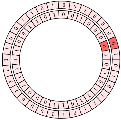
Suppose we take one LFSR output and duplicate it, with one instance delayed. We end up with two sequences that have low correlation for a shift of zero, and can visualize it as a pair of circular tracks, shown below for the quotient ring $ GF(2)[x]/{p_1(x)} $ for $ p_1(x) = x^5+x^2+1 $:

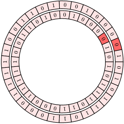
(The darker sector in each track shows the initial value of the LFSR with 00001 state, so it’s easy to tell how much one sequence has been delayed relative to the other.)

Unfortunately, since they are the same underlying sequence, there is a position where the sequences line up, and in this case the correlation is very high.

With Gold codes, we use two quotient rings; $ GF(2)[x]/{p_1(x)} $ and $ GF(2)[x]/{p_3(x)} $ with $ p_3(x) = x^5 + x^4 + x^3 + x^2 + 1 $ resulting from decimating the first sequence by a factor of 3.

Below are two pairs of tracks; the red tracks are from $ p_1(x) $ and the green tracks are from $ p_3(x) $. Each output sequence represents the XOR combination of a red track and a green track, but we use different relative delays between the red and green track.

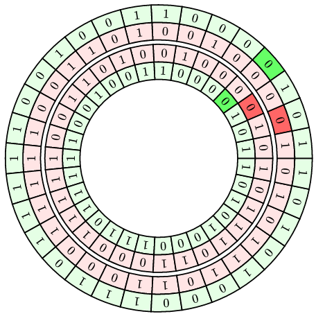
In this case, there’s no way to line them up; if the green tracks line up, then the red tracks are still misaligned, and if the red tracks line up, then the green tracks are misaligned.

We are effectively “keying” the output sequence of a Gold code, by controlling the relative shift value between the two components, and cyclic rotation of the output sequence cannot change that shift value.

This doesn’t explain how we can maintain low correlation across the entire cross-correlation function (that needs math), but it does show how we can avoid high correlation.

Spread-Spectrum Showcase with Gold Codes

Let’s try it in practice, using the same kind of technique as in Part XII.

# functions from part XII
# (recv_uart_dss has been edited slightly)

pi = np.pi
def cos2pi(t):
    return np.cos(2*pi*t)
def smod(x,n):
    return (((x/n)+0.5)%1-0.5)*n
def flatcos(t):
    y = (cos2pi(t) - cos2pi(3*t)/6) / (np.sqrt(3)/2)
    y[abs(smod(t,1.0)) < 1.0/12] = 1
    y[abs(smod(t-0.5,1.0)) < 1.0/12] = -1
    return y
def error_count(msg1, msg2):
    errors = 0
    for c1,c2 in zip(msg1, msg2):
        if c1 != c2:
            errors += 1
    return errors

def uart_bitstream(msg, Nsamp, idle_bits=2, smooth=True):
    """
    Generate UART waveforms with Nsamp samples per bit of a message.
    Assumes one start bit, one stop bit, two idle bits.
    """
    bitstream = []
    b_one  = np.ones(Nsamp)
    b_zero = b_one*-1
    bprev = 1
    if smooth:
        # construct some raised-cosine transitions
        t = np.arange(2.0*Nsamp)*0.5/Nsamp
        w = flatcos(t)
        b_one_to_zero = w[:Nsamp]
        b_zero_to_one = w[Nsamp:]
    def to_bitstream(msg):
        for c in msg:
            yield 0        # start bit
            c = ord(c)
            for bitnum in xrange(8):
                b = (c >> bitnum) & 1
                yield b
            yield 1        # stop bit
        for _ in xrange(idle_bits):
            yield 1
    for b in to_bitstream(msg):
        if smooth and bprev != b:
            # smooth transitions
            bitstream.append(b_zero_to_one if b == 1 else b_one_to_zero)
        else:
            bitstream.append(b_one if b == 1 else b_zero)
        bprev = b
    x = np.hstack(bitstream)
    t = np.arange(len(x))*1.0/Nsamp
    return pd.Series(x,t,name=msg)

def receive_uart_dsss(bitstream, pn, Nsamp, initial_state=1,
                     return_raw_bits=False):
    N = len(bitstream)
    if pn is None:
        xr = bitstream
    elif isinstance(pn, GF2QuotientRing):
        field = pn
        s = np.array(list(lfsr_output(field, 
                                      initial_state=initial_state,
                                      nbits=N)))*2-1
        xr = bitstream*s
    else:
        xr = bitstream * pn
    # Integrate over intervals:
    #   - cumsum for cumulative sum
    #   - decimate by Nsamp
    #   - take differences
    #   - skip first sample
    xbits = (xr.cumsum().iloc[::Nsamp].diff()/Nsamp).shift(-1).iloc[:-1]
    if return_raw_bits:
        return xbits
    #   - test whether positive or negative, convert to 0 or 1
    xbits = (xbits > 0).values*1
    # now take each stretch of 10 bits, 
    # grab the middle 8 to drop the start and stop bits,
    # and convert to an ASCII coded character 
    msg = ''
    for k in xrange(0,10*(len(xbits)//10),10):
        bits = xbits[k+1:k+9]
        ccode = sum(bits[j]*(1<<j) for j in xrange(8))
        msg += chr(ccode)
    return msg

# Step 1: construct the messages

messages = """-----
But our fish said, "No! No!
Make that cat go away!
Tell that cat in the hat
you do NOT want to play.
He should not be here.
He should not be about.
He should not be here
when your mother is out!"
-----
I do not like them
In a house.
I do not like them
With a mouse.
I do not like them
Here or there.
I do not like them
Anywhere.
I do not like green eggs and ham.
I do not like them, Sam-I-am.
-----
I am the very model of a modern Major-General,
I've information vegetable, animal, and mineral,
I know the kings of England, and I quote the fights historical
From Marathon to Waterloo, in order categorical;
I'm very well acquainted, too, with matters mathematical,
I understand equations, both the simple and quadratical,
About binomial theorem I'm teeming with a lot o' news,
With many cheerful facts about the square of the hypotenuse.
-----
'Twas brillig, and the slithy toves
Did gyre and gimble in the wabe:
All mimsy were the borogoves,
And the mome raths outgrabe. 

"Beware the Jabberwock, my son!
The jaws that bite, the claws that catch!
Beware the Jubjub bird, and shun
The frumious Bandersnatch!
-----
"The time has come," the Walrus said,
"To talk of many things:
Of shoes---and ships---and sealing-wax---
Of cabbages---and kings---
And why the sea is boiling hot---
And whether pigs have wings."
-----
Just sit right back
And you'll hear a tale
A tale of a fateful trip,
That started from this tropic port,
Aboard this tiny ship.
The mate was a mighty sailin' lad,
The skipper brave and sure,
Five passengers set sail that day,
For a three hour tour,
A three hour tour.
-----
Here's the story
Of a lovely lady
Who was bringing up three very lovely girls
All of them had hair of gold
Like their mother
The youngest one in curls
-----
Then this ebony bird beguiling my sad fancy into smiling,
By the grave and stern decorum of the countenance it wore,
"Though thy crest be shorn and shaven, thou," I said, "art sure no craven,
Ghastly grim and ancient Raven wandering from the Nightly shore—
Tell me what thy lordly name is on the Night's Plutonian shore!"
            Quoth the Raven "Nevermore."
-----"""

messages = [msg.strip() for msg in messages.split("-----") if msg != '']
max_msglen = max(len(msg) for msg in messages)
# pad messages to their maximum length
def pad(msg, L, nspace=64):
    for k in xrange(len(msg), L):
        msg += '\n' if (k % nspace) == 0 else ' '
    return msg
messages = [pad(msg, max_msglen) for msg in messages]

# Step 2: create Gold sequences for each, then use to encode the messages

def eval_mutual_correlations(sequences):
    """
    Returns a measure of the sum of correlations between all pairs of sequences 
    """
    nseq = len(sequences)
    S = 0
    for b in xrange(1,nseq):
        for a in xrange(b):
            s = (sequences[a]*sequences[b]).sum()
            S += abs(s)
    return S

def find_random_worstcase_correlation(sequences, period, ntries):
    """
    Returns offsets that will make the sum of correlations 
    as high as possible, given some number "ntries" attempts.
    
    We do this to make sure we're not accidentally making it easy on ourselves.
    """
    worst_S = 0
    worst_phases = None
    nseq = len(sequences)
    for _ in xrange(ntries):
        phases = np.random.randint(0,period,nseq)
        sequences2 = [np.roll(seq[:period],phase) for seq,phase in zip(sequences,phases)]
        S = eval_mutual_correlations(sequences2)
        if S > worst_S:
            worst_S = S
            worst_phases = phases
    return worst_S, worst_phases

def create_transmitter_sequences(nchars, field1, field2, trange, 
                                 Nsamples_per_bit, verbose=True):
    nbits = Nsamples_per_bit * 10 * nchars
    if verbose:
        print(("Generating %d bits of pseudonoise\n"+
              "(enough to cover %d bytes via UART at %d samples per bit)")
              % (nbits, nchars, Nsamples_per_bit))

    # First find the sequences synchronized in time (no delay)
    transmitter_sequences = [gold_sequence(field1, field2, t, nbits=nbits)
                             for t in trange]

    # Then find a more devious set of delays -- we want to find one with
    # a worse correlation
    period = (1<<field1.degree) - 1
    S, phases = find_random_worstcase_correlation(transmitter_sequences, period, ntries=100)

    transmitter_sequences = [gold_sequence(field1, field2, t, nbits=nbits, delay=delay)
                             for t,delay in zip(trange, phases)]
    S_verify = eval_mutual_correlations([s[:period] for s in transmitter_sequences])
    assert S == S_verify
    return transmitter_sequences

# Create a combined message V which is the sum of all transmitted messages.
# Then see if we can decode each of them.

def try_encoding(messages, transmitter_sequences, Nsamples_per_bit):
    umessages = [uart_bitstream(message, Nsamples_per_bit, idle_bits=0, smooth=False)
                 for message in messages]
    return [umessage*pn for umessage,pn in zip(umessages, transmitter_sequences)]

def try_decoding(encoded_messages, messages, transmitter_sequences, Nsamples_per_bit):
    for msgnum, message in enumerate(messages):
        received_message = receive_uart_dsss(encoded_messages, 
                                             transmitter_sequences[msgnum],
                                             Nsamples_per_bit)
        print "msgnum=%d: %d errors" % (msgnum, error_count(message, received_message))
        print received_message

SR = 128
np.random.seed(12345)
transmitter_sequences = create_transmitter_sequences(
                            max_msglen,
                            qr1, qr3,
                            trange = xrange(-2,6),
                            Nsamples_per_bit = SR)        
V = sum(try_encoding(messages, transmitter_sequences, Nsamples_per_bit=SR))
try_decoding(V, messages, transmitter_sequences, Nsamples_per_bit=SR)

Generating 560640 bits of pseudonoise
(enough to cover 438 bytes via UART at 128 samples per bit)
msgnum=0: 0 errors
But our fish said, "No! No!
Make that cat go away!
Tell that cat in the hat
you do NOT want to play.
He should not be here.
He should not be about.
He should not be here
when your mother is out!"                                                             
                                                               
                                                               
                                                    
msgnum=1: 0 errors
I do not like them
In a house.
I do not like them
With a mouse.
I do not like them
Here or there.
I do not like them
Anywhere.
I do not like green eggs and ham.
I do not like them, Sam-I-am.  
                                                               
                                                               
                                                               
                                                    
msgnum=2: 0 errors
I am the very model of a modern Major-General,
I've information vegetable, animal, and mineral,
I know the kings of England, and I quote the fights historical
From Marathon to Waterloo, in order categorical;
I'm very well acquainted, too, with matters mathematical,
I understand equations, both the simple and quadratical,
About binomial theorem I'm teeming with a lot o' news,
With many cheerful facts about the square of the hypotenuse
msgnum=3: 0 errors
'Twas brillig, and the slithy toves
Did gyre and gimble in the wabe:
All mimsy were the borogoves,
And the mome raths outgrabe. 

"Beware the Jabberwock, my son!
The jaws that bite, the claws that catch!
Beware the Jubjub bird, and shun
The frumious Bandersnatch!                                                         
                                                               
                                                    
msgnum=4: 0 errors
"The time has come," the Walrus said,
"To talk of many things:
Of shoes---and ships---and sealing-wax---
Of cabbages---and kings---
And why the sea is boiling hot---
And whether pigs have wings."                                                             
                                                               
                                                               
                                                    
msgnum=5: 0 errors
Just sit right back
And you'll hear a tale
A tale of a fateful trip,
That started from this tropic port,
Aboard this tiny ship.
The mate was a mighty sailin' lad,
The skipper brave and sure,
Five passengers set sail that day,
For a three hour tour,
A three hour tour.                                                     
                                                               
                                                    
msgnum=6: 0 errors
Here's the story
Of a lovely lady
Who was bringing up three very lovely girls
All of them had hair of gold
Like their mother
The youngest one in curls                                          
                                                               
                                                               
                                                               
                                                    
msgnum=7: 0 errors
Then this ebony bird beguiling my sad fancy into smiling,
By the grave and stern decorum of the countenance it wore,
"Though thy crest be shorn and shaven, thou," I said, "art sure no craven,
Ghastly grim and ancient Raven wandering from the Nightly shore—
Tell me what thy lordly name is on the Night's Plutonian shore!"
            Quoth the Raven "Nevermore."

Perfect! Eight messages all coexisting in lovely spread-spectrum harmony, by modulating with different Gold codes and adding them together. And we could decode all eight of them without error. We did that with a spreading ratio of 128 (chip rate of 128 times the bit rate). Let’s try it with 64:

SR = 64
transmitter_sequences = create_transmitter_sequences(
                            max_msglen,
                            qr1, qr3,
                            trange = xrange(-2,6),
                            Nsamples_per_bit = SR)

V = sum(try_encoding(messages, transmitter_sequences, Nsamples_per_bit=SR))
try_decoding(V, messages, transmitter_sequences, Nsamples_per_bit=SR)

Generating 280320 bits of pseudonoise
(enough to cover 438 bytes via UART at 64 samples per bit)
msgnum=0: 6 errors
But our fish said, "No! No!
Make that cat go away!
Tell that cat in the hat
yOu do NOT want to play.
He should not be here.
He should n/t be about.
He should not be here
when your mothep is out!"                 `                                    `      
                                                               
                                                       0       
                                                    
msgnum=1: 7 errors
I do nmt like them
In a house,
I do not like them
With a mouse.
I do not like them
Here or there.
I do not like them
Anywhere.
I do not like green eggs and ham.
I do not like them, Sam-I-am.  
            !                 "                                
                 0    !                                        
                                                               
                     0                              
msgnum=2: 7 errors
I am the very model of a modern Major-General,
I've information vegetable, animal, and mineral,
I know the kings of England, and I quote the fights historical
From Marathon to Waterloo, in order citegorical;
I'm very well acquainted, too, with matTers mathematical,
I understAnd equations, both the�simple and quadratical,
About binomial theorem I'm teeming with a lot o' neWs,
With many cheerful fagts about the square of th� hypotenuse
msgnum=3: 9 errors
'Twas brillig, and the slithy toves
Did gyre and gimble in the wabe:
Al� mymsy were the borogoves,
And the mome raths outgrabe. 

 Bewarethe Jabberwock, my son!
The jaws that bite, the claws that catch!
Beware the Jubjub bird, and shun
The fruoious Bandersnatch!                                                        
                                                           0   
                                             `     
msgnum=4: 5 errors
"The time has come," the Walrus said,
"To talk of many things:
Of shoes---and ships---and sealing-wax---
Of cabbages---and kings---
And why the sea is bOiling hot---
And whether pigs have wings."        �          (                                         
        (                                        "             
                                                               
                                                    
msgnum=5: 4 errors
Just sit right back
And you'll hear a tale
A tale of a fateful trip,
That started from this tro`ic port,
Aboard this tiny ship.
The mate was a mighty sailin' lad,
The skipper brave and sure,
Five passengers sep sail that day,
For a three hour tour,
@ three hour tour.                                                     
                                                               
              (                                     
msgnum=6: 8 errors
Here's the story
Of a lovely lady
Who was bringing up three verx lovely girls
All"of them had hair of gold
Like their mo|her
The youngest one in curls                                         
                                                               
                                                               
                                $              $               
                                  0                
msgnum=7: 7 errors
Then this ebony bird beguiling my sad fancy into smili~g,
By the grave and stern decorum of the countenance ht wore,
"Though thy crest be shorn and shaven, thou," I said, "art sure no craven,
Ghastly grim and anc�ent Raven wanderilg from the Nightly shore—
Tell me what thy lordly name is on the Night's Plutonian sjore!"
            Quoth the Raven "Nevermore."    (

Well, that didn’t quite work; a spreading ratio of 64 isn’t enough for eight messages to coexist in spread-spectrum harmony. We can choose fewer messages:

SR = 64
transmitter_sequences = create_transmitter_sequences(
                            max_msglen,
                            qr1, qr3,
                            trange = xrange(-2,6),
                            Nsamples_per_bit = SR)
nmsg = 5
V = sum(try_encoding(messages[:nmsg], transmitter_sequences[:nmsg], Nsamples_per_bit=SR))
try_decoding(V, messages[:nmsg], transmitter_sequences[:nmsg], Nsamples_per_bit=SR)

Generating 280320 bits of pseudonoise
(enough to cover 438 bytes via UART at 64 samples per bit)
msgnum=0: 0 errors
But our fish said, "No! No!
Make that cat go away!
Tell that cat in the hat
you do NOT want to play.
He should not be here.
He should not be about.
He should not be here
when your mother is out!"                                                             
                                                               
                                                               
                                                    
msgnum=1: 0 errors
I do not like them
In a house.
I do not like them
With a mouse.
I do not like them
Here or there.
I do not like them
Anywhere.
I do not like green eggs and ham.
I do not like them, Sam-I-am.  
                                                               
                                                               
                                                               
                                                    
msgnum=2: 0 errors
I am the very model of a modern Major-General,
I've information vegetable, animal, and mineral,
I know the kings of England, and I quote the fights historical
From Marathon to Waterloo, in order categorical;
I'm very well acquainted, too, with matters mathematical,
I understand equations, both the simple and quadratical,
About binomial theorem I'm teeming with a lot o' news,
With many cheerful facts about the square of the hypotenuse
msgnum=3: 0 errors
'Twas brillig, and the slithy toves
Did gyre and gimble in the wabe:
All mimsy were the borogoves,
And the mome raths outgrabe. 

"Beware the Jabberwock, my son!
The jaws that bite, the claws that catch!
Beware the Jubjub bird, and shun
The frumious Bandersnatch!                                                         
                                                               
                                                    
msgnum=4: 0 errors
"The time has come," the Walrus said,
"To talk of many things:
Of shoes---and ships---and sealing-wax---
Of cabbages---and kings---
And why the sea is boiling hot---
And whether pigs have wings."

We can get a sense of the success rate by looking at the statistics of received bits using the Gold code of one message to decode some number K of messages encoded with other Gold codes.

enc_messages = try_encoding(messages, transmitter_sequences, Nsamples_per_bit=SR)

import matplotlib.pyplot as plt
import pandas as pd
%matplotlib inline

# Plot received noise as time series
M = 0
noise_of_others = []
for K in xrange(1,8):
    M += enc_messages[K]
    msgr = receive_uart_dsss(M, pn=transmitter_sequences[0], Nsamp=SR, return_raw_bits=True)
    noise_of_others.append(msgr)
    
fig = plt.figure()
ax = fig.add_subplot(1,1,1)
for K in xrange(7,0,-1):
    msgr = noise_of_others[K-1]
    ax.plot(msgr,drawstyle='steps-post',linewidth=0.8,label='K=%d'%K)
ax.legend(labelspacing=0, fontsize=10)
ax.set_title('"Noise" seen by one transmitter after decoding sum of other signals',
            fontsize=11)

# Now let's show histograms

bins = np.arange(-15,15)*0.1

fig = plt.figure()
ax = fig.add_subplot(1,1,1)
stats = []
for K in xrange(7,0,-1):
    msgr = noise_of_others[K-1]
    stdev = np.std(msgr)
    peak = np.max(np.abs(msgr))
    stats.append(dict(K=K,stdev=stdev,peak=peak))
    ax.hist(msgr, bins=bins,
            label='K=%d $\\sigma=$%.3f, pk=%.3f' % (K,stdev,peak),
            histtype='step')
ax.legend(labelspacing=0, fontsize=8)
ax.set_title('Histogram of "noise" seen by one transmitter from other signals',
            fontsize=11)

# Summary statistics as a function of K
fig = plt.figure()
ax = fig.add_subplot(1,1,1)
df = pd.DataFrame(stats).set_index('K').sort_index()
df.plot(ax=ax, style=['.','+'])
xlim = (0.9,7.1)
xfit = np.linspace(xlim[0],xlim[1],100)
for f in ['stdev','peak']:
    p = np.polyfit(df.index,df[f],1)
    ax.plot(xfit, np.polyval(p,xfit))
ax.set_xlim(0.9,7.1)
ax.set_title('Summary statistics of received "noise" as a function of K');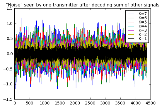

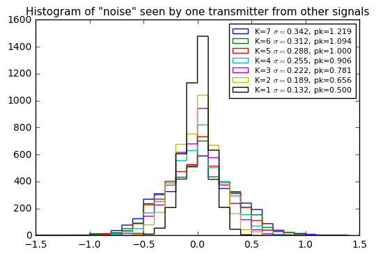
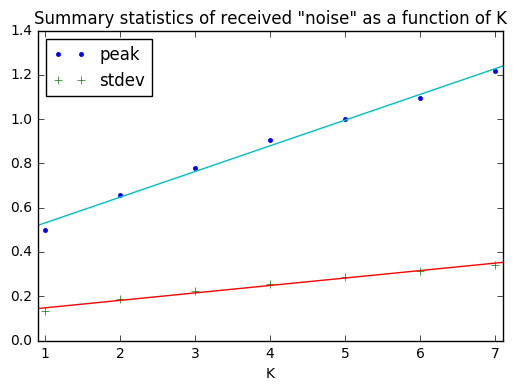
The weird thing here is that the peak and standard deviation of the “noise” observed by one transmitter trying to decode encoded signals from other transmitters, seem to increase linearly (with an offset) as a function of the number of other transmitters.

If I had some number K of transmitters of true Gaussian noise with identical amplitudes, and the noise was uncorrelated, I would expect the peak values and standard deviations to add in quadrature — that is, 4 signals should have twice the standard deviation of 1, 9 signals should have three times the standard deviation of 1 signal, and so forth.

So a linear increase is odd; either I’ve screwed up my math somewhere, or it’s a sign that multiple signals have some sign of correlation. Perhaps an astute reader can help explain this phenomenon.

Dueling Signals: Common PRBS vs. Gold Codes

One more empirical test: let’s look at the case of only two transmitters. The whole reason for using Gold codes was for us to be able to assign a PRBS to a whole bunch of transmitters so that any two of them would have low mutual cross-correlation.

If there are only two transmitters, I can pick a “preferred pair” of polynomials and use the resulting maximal-length PRBS for each transmitter, and have the same kind of performance as with Gold codes — after all, these maximal-length PRBS, withough XORing together, are two special cases of a Gold code.

If there are only two transmitters and they are synchronized in chip rate so that they maintain some desired phase distance, we can tolerate using the same 15-bit maximal length LFSR for both transmitters. Since the period is 32767 chips, the best choice is to increase phase spacing to the maximum of 16383, so that we can tolerate a relative delay in impulse response of 16383: one transmitter could be very far away and one close up, or we just have a system with a lot of filtering for some reason.

Let’s see how these cases compare. We’ll use spread-spectrum encoding on a signal from one transmitter, and see how much interference we get when decoded with the PRBS of another transmitter.

SR = 64
msgbits = uart_bitstream(messages[0], SR, idle_bits=0, smooth=False)
nbits = len(msgbits)
prbs_common = pnr(qr1,nbits=nbits,delay=0)
# Use pseudonoise from the other member of the preferred pair,
# but with a delay so that we get worst-case cross-correlation (and not -1)
for d in xrange(100):
    prbs_gold = pnr(qr3,nbits=nbits,delay=0)
    S = sum(prbs_common[:32767] * prbs_gold[:32767])
    if S != -1:
        break
print "d=",d, "S=",S

# Verify that the autocorrelation property is still true for prbs_common
R = circ_correlation_fft(prbs_common[:32767], prbs_common[:32767],
                        result_type=int)
print "R=",R
assert (R[1:] == -1).all()

d= 0 S= 255
R= [32767    -1    -1 ...,    -1    -1    -1]

def compare_recv_noise(msgbits, pnlist, pnref, SR, labels, bins=None):
# Encode the same message both ways:
#   - with the same PRBS, shifted by 16383
#   - with another PRBS from the preferred pair, with worst-case correlation

    E = [msgbits * pn for pn in pnlist]
    recv_noise = [receive_uart_dsss(M, 
                                    pn=pnref, 
                                    Nsamp=SR, 
                                    return_raw_bits=True)
                  for M in E]

    fig = plt.figure()
    ax = fig.add_subplot(1,1,1)
    for k,label in enumerate(labels):
        msgr = recv_noise[k]
        stdev = np.std(msgr)
        peak = np.max(np.abs(msgr))
        ax.hist(msgr, bins=bins,
                label='%s $\\sigma=$%.4f, pk=%.4f' % (label,stdev,peak),
                histtype='step')
    ax.legend(labelspacing=0, fontsize=8, loc='best');
    ax.set_title("Decoded received 'noise', samples per bit = %d" % SR)
    
compare_recv_noise(msgbits, 
                   pnlist=[np.roll(prbs_common, 16383), prbs_gold],
                   pnref=prbs_common,
                   SR=SR,
                   labels=['common','Gold'],
                   bins = np.arange(-12,12)*0.04)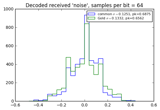

There’s really not much difference here. This is probably due to the fact that the LFSR period is 32767, but we’re using 64 samples of pseudonoise per bit, so we don’t get the benefit of a correlation of pseudonoise over its entire period; that’s where the ultralow autocorrelation of a PRBS comes into play. Let’s try doing that instead, with a short message:

msg = "This is a test of the emergency pseudonoise system."
SR = 32767
msgbits = uart_bitstream(msg, SR, idle_bits=0, smooth=False)
nbits = len(msgbits)

prbs_common = pnr(qr1,nbits=nbits,delay=0)
prbs_gold = pnr(qr3,nbits=nbits,delay=d)
print "d=",d,"S=",sum(prbs_common[:32767]*prbs_gold[:32767])

compare_recv_noise(msgbits, 
                   pnlist=[np.roll(prbs_common, 16383), prbs_gold],
                   pnref=prbs_common,
                   SR=SR,
                   labels=['common','Gold'],
                   bins = np.arange(-50,50)*0.0005
                   )

d= 0 S= 255

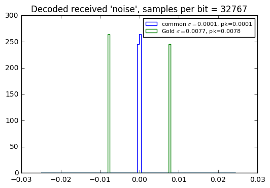
Yeah, the use of a common PRBS (used with synchronous frequency) has smaller interference error than use of Gold codes, when used with a full period, namely when the spreading ratio equals the PRBS period.

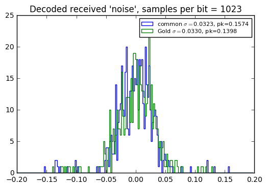
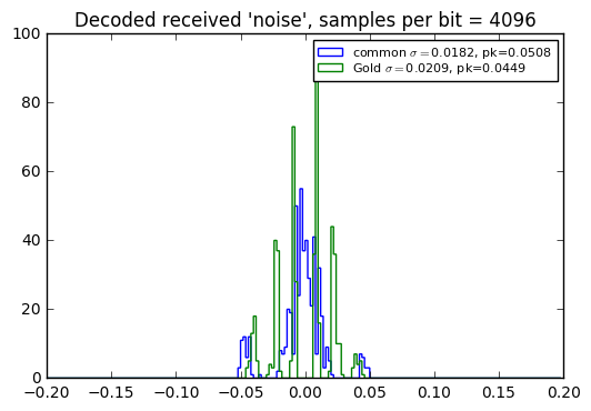
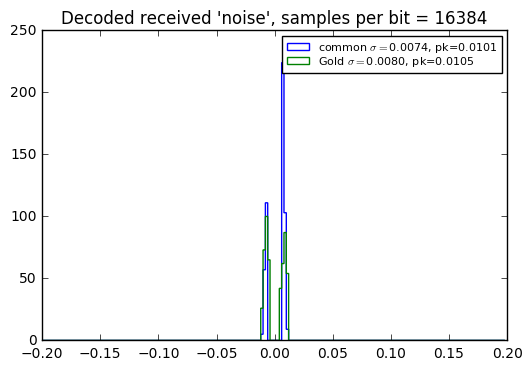
When used with an incomplete period, there’s no significant difference in received interference level, as shown in the error histograms below… which leads me to conclude that in most situations, it’s a better choice to use Gold codes, which then have the advantage that they can be used asynchronously.

Note also that a larger number of PRBS samples per bit yields lower interference level, which makes sense, since the spreading ratio is higher.

msg = "This is a test of the emergency pseudonoise system."
for SR in [1023, 4096, 16384]:
    msgbits = uart_bitstream(msg, SR, idle_bits=0, smooth=False)
    nbits = len(msgbits)

    prbs_common = pnr(qr1,nbits=nbits,delay=0)
    prbs_gold = pnr(qr3,nbits=nbits,delay=d)
    S = sum(prbs_common[:32767]*prbs_gold[:32767])
    assert abs(S) > 1

    compare_recv_noise(msgbits, 
                       pnlist=[np.roll(prbs_common, 16383), prbs_gold],
                       pnref=prbs_common,
                       SR=SR,
                       labels=['common','Gold'],
                       bins = np.arange(-100,100)*0.002
                       )

Use of Gold Codes in the Global Positioning System (GPS)

Gold codes, along with similar constructions called Kasami codes (which are similar to Gold codes but, if I understand them correctly, also allow for decimations as well as shifts in order to create a larger set of mutually low-correlation sequences… and since that’s about all that I know about them, I won’t mention them again) are widely used in asynchronous CDMA systems. One of these is the USA’s Global Positioning System, or GPS, as we have come to know it. The fact that we can use a receiver to tell where we are in the world, just by receiving and processing satellite signals, is a triumph of engineering, and it has become ubiquitous enough that we don’t even think twice when we can use a smart phone to find directions or play bizarre augmented reality games.

Satellite-based navigation systems have been around since the early 1960’s, starting with TRANSIT, but the 1973 kickoff of GPS (then known as the Defense Navigation Satellite System) by the US military benefited from two technological innovations of the 1960s: rubidium (and later cesium) atomic clocks, and Gold codes. The first GPS satellite launched in 1978 and a full constellation was achieved in the mid-1990s, although even civilian use started early on, with a trans-Atlantic flight carefully planned and executed in 1983 from Cedar Rapids, Iowa, to LeBourget, France, using GPS navigation, broken into five segments over four days to allow sufficient satellite visibility during each flight segment.

The interface specification for GPS that covers the use of Gold codes is IS-GPS-200. The signal transmitted by each of the GPS satellites includes several modulating sequences, including a Coarse Acquisition or C/A code specific to the satellite, and a P and Y code for precision navigation and encryption. (The encryption aspect was known as Selective Availability, and intentionally degraded performance for nonmilitary users, until May 2000 when President Clinton directed that this degradation be turned off.)

An overall block diagram (Figure 3-1 of IS-GPS-200H) is shown below:

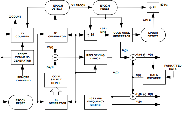
The C/A code is based on a subset of Gold codes using 10-bit LFSRs, with a chip rate of precisely 1.023MHz; the resulting PRBS repeats exactly once per millisecond. The LFSRs are Fibonacci implementations (feedback using the XOR of several bits, rather than the Galois implementation that XORs the output bit into several state bits) using polynomials $ x^{10} + x^3 + 1 $ and $ x^{10} + x^9 + x^8 + x^6 + x^3 + x^2 + 1 $, shown below (from Figure 3-10)

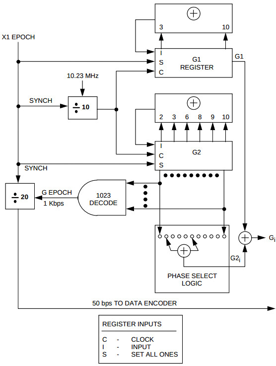
Instead of arbitrary Gold codes, the specification mandates that the output bits are derived from an XOR of exactly two of the state bits, and the possible combinations are listed in tables like the one below (Table 3-1a):

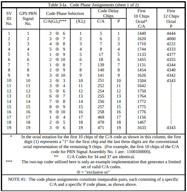
I’m not sure why this two-tap approach was used; an equivalent approach would have been to use Galois implementations and load in a particular pattern into the shift register upon an “epoch reset” event.

Each satellite uses a different Gold code, and the relatively short period (n=1023 chips) allows for both synchronization and spread-spectrum gain, so that the precision code can then be used to determine the relative transmission distances between different satellites, and thereby (through a lot of geometry and signal processing that I don’t understand well enough to present, and this article is long enough anyway) determine the receiver’s position.

The actual data bits from the satellites are sent at 50Hz, which allow the Gold codes to repeat their entire sequence 20 times for each data bit.

The P-code is also LFSR-based, and has a chip rate of precisely 10.23MHz, but is “short-cycled” (reset before the natural cycle completes) to determine a repeat rate of exactly 1.5 seconds or 15345000 chips.

What I think is really neat about GPS, is that it is theoretically possible to take a radio receiver and ADC digitizing at 10.23MHz and use DSP techniques to decode the spread-spectrum and recover the messages from various satellites. This is a software-defined radio (SDR) approach, and if I ever get into SDR, then this would be the application I’d want to pursue, along with the position recovery using Kalman filters. In practice, most of this stuff is already done for you in GPS chipsets, at various levels. But the technology is fairly understandable, on the level of the articles in this series; you don’t have to have a PhD in the mathematics of finite fields to understand how it works.

Wrapup

We covered a number of aspects of Gold codes today:

Schrödinger’s Highway: asynchronous behavior can result in worst-case synchronous behavior as signals go in and out of phase, so using a common PRBS for multiple spread-spectrum transmitters requires synchronization in frequency to maintain sufficient phase separation.
Path delays and the $ O(N^2) $ increase in pairs of transmitters makes it impractical to use a common PRBS, even with synchronization, unless the period is very large.
So-called “preferred pairs” of PRBS can be constructed to produce a three-valued cross-correlation function that achieves minimal cross-correlation.
Gold codes are constructed from a preferred pair by XORing one PRBS with various shifts of the other PRBS.
We showed an example of combining eight encoded messages, each using a different Gold code, where each message could be decoded without significant interference from the others.
There is no significant difference in received interference level, between using Gold codes, and using a common PRBS, for spread-spectrum encoding, if the number of samples per bit is not a complete period. If we do use a complete period of the PRBS for each bit, then using a common PRBS produces lower interference level due to its ultralow autocorrelation function.
The Global Positioning System uses Gold codes for the Coarse Acquisition (C/A) spreading sequence.

In my next article in this series, we’re going to look at error-detecting codes and error-correcting codes.

References

Robert Gold, Optimal Binary Sequences for Spread Spectrum Multiplexing, IEEE Trans. on Information Theory vol. IT-13 pp. 619-621 Oct 1967. This is ground zero for Gold codes, a short, mathematical paper in the correspondence section of IEEE Transactions on Information Theory. Gold was working for Magnavox Research Laboratories at the time. Yes, that Magnavox. At one point in time, electronics companies had research labs and they produced golden eggs like this one.
Robert McEliece, Finite Fields for Computer Scientists and Engineers, Kluwer Academic Publishers, 1987. This is one of those books that is hard to get and expensive, yet useful. The title, however, is misleading — it sounds like it is going to make finite fields accessible and practical, but will steer clear of the thicket of proofs and hardcore mathematics. It does not. I do like it more than Lidl & Niederreiter, however. And it has a whole chapter on “Crosscorrelation Properties of m-sequences”.
Dilip V. Sarwate and Michael B. Pursley, Cross-correlation Properties of Pseudorandom and Related Sequences, Proceedings of the IEEE vol. 68 no. 5 pp. 593-618 May 1980.

Thanks also to Dr. Dilip Sarwate for answering a question I had about why Gold and Kasami codes are used.

Global Positioning System

Global Positioning Systems Directorate Systems Engineering and Integration: Interface Specification IS-GPS-200, United States Air Force, September 2013 (Revision H).
GPS Basics, Sparkfun.com
The Origins of GPS, and the Pioneers Who Launched the System, GPS World, May 2010.
The Origins of GPS, Fighting to Survive, GPS World, June 2010.
David L. van Dusseldorp, Historic GPS Flight in 1983 Hinted at Today’s Innovations, GPS Solutions, Vol 1, Issue 4, 1996.
Stefan Wallner and José Ángel Ávila-Rodríguez, Codes: The PRN Family Grows Again, Inside GNSS, September/October 2011.

Appendix: How Did We Calculate Traffic Density?

In the Schrödinger’s Highway example, I came up with a value of about 50% for widthwise density and 6% for the lengthwise density of traffic just prior to congestion. I hate giving numbers without a justification where they came from, but in this case it would have interrupted the article, so in case you’re curious how I came up with those numbers, here’s how.

(My assumptions were that this is in the western USA, with typical USA highway widths, and speeds on the order of 120km/hr ≈ 75 MPH, so these numbers may be a little bit different elsewhere in the world.)

As for width — this is easy; a few years ago I wrote an article on design margin that used an example of lane widths on US interstate highways. AASHTO design standards state that the minimum lane width is to be 3.6m. Not including mirrors, most US cars are in the 1.7-1.9m width range. So let’s use 1.8m, meaning that the width density is about 50%.

Length is a bit tougher.

Traffic flow data looks something like this:

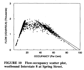
This graph is showing the relationship between two variables. One of them (the x-axis) is called occupancy, and it’s the density along a lane of traffic. Many highways have inductive loop detectors for measuring traffic flow, and they’re arranged in banks at various points, shown below schematically as little squares. The occupancy is defined as the fraction of time that the loop detector senses a vehicle.

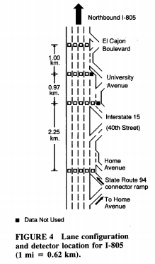
Both of these figures are from a 1993 Transportation Research Record article by Paul Hsu and James Banks called Effects of Location on Congested-Regime Flow-Concentration Relationships for Freeways. Just a little light reading.

The y-axis of the graph measures traffic flow, defined as the number of vehicles per lane that passes a given point, per unit time. If we increment a counter every time the loop detector senses a vehicle, then we can count the number of vehicles per hour in that lane.

On the left side of this graph, we’ve got very linear behavior that relates to the length of a typical car and the speed it’s going. Typical cars are between 3.8m - 5.5m in length. Let’s say we have a bunch of cars which are 4.7m long. And they’re going 120km/hr (74.56 mph). If these cars could go bumper-to-bumper at that speed — which is not going to happen — then the flow rate would be 120km/hr divided by 4.7m = about 25500 cars per hour. Not gonna happen. But it tells you the theoretical limit, and if we had 1% occupancy then the flow rate would be 255 cars per hour; 2% occupancy would be 510 cars per hour, and so on. (The graph from Hsu and Banks shows 1000 cars per second at 10% occupancy, so either this stretch of highway has a much slower speed, or there are a lot of trucks and trailers, or perhaps I’m missing something else.)

The reason we don’t get to 100% occupancy at full speed is it’s not safe; even if we weren’t scared, our reaction time is too slow, and the chance of accidents would be 100%. In practice, our following distance is 1.5-2 seconds, meaning that for every 1m/s = 3.6km/hr the car is traveling, we’d need 2m distance between cars to feel comfortable so that we could stop before hitting the car in front of us. (Remember the two-second rule?) Travel twice as fast, you need twice the distance. The cars can’t get denser unless they slow down to maintain a safe distance, and as a result there is a maximum traffic flow. It’s not 100% occupancy. At 120km/hr = 33.33m/s, with a two-second following distance, that means there would need to be 66.67m distance between cars. With 4.7m cars, that’s only 4.7 / (4.7 + 66.7) = 6.58% occupancy, which translates to 25500 × 6.58% = 1780 cars/second. The graph from Hsu and Banks shows scattering in the 1200-2000 cars/second range as a limit, so we’re in the right ballpark. If we define congestion as the point at which traffic slows down to 95% of its free-flowing speed, then this is 0.95 × 120km/hr = 114km/hr, and 0.95 × 6.58% = 6.25% occupancy.

Anyway, we’re talking about 6.25% occupancy at the point of congestion at 120km/hr. So that’s our lengthwise density. Multiply by 50% width density and we’re only using up 3.1%, or 1/32, of the highway area with vehicles. We can cover more of that area, but not without introducing congestion that slows down traffic (for higher lengthwise density) or that risks side-to-side collisions (for higher width density).

All this, just because we don’t want to hit another car. Sheesh. As the occupancy ratio goes up, we go from fun cruising to metal-on-metal contact, with a bunch of stress and fear towards the end. We can’t just drive at whatever speed we like; once congestion occurs, the cars have to synchronize their speeds and have sufficient spacing between them.

By the way, bonus points to anyone who guesses where I took those landscape pictures.

You might also like... (promoted content)

Check out Memfault's New Sandbox!

The 2024 Embedded Online Conference - Register Early and Save with Promo Code ER2024!

Comments

Comments
Write a Comment

Select to add a comment

To post reply to a comment, click on the 'reply' button attached to each comment. To post a new comment (not a reply to a comment) check out the 'Write a Comment' tab at the top of the comments.

Please login (on the right) if you already have an account on this platform.

Otherwise, please use this form to register (free) an join one of the largest online community for Electrical/Embedded/DSP/FPGA/ML engineers:

Choose a Username

E-Mail (Work, School or ieee)

First Name

Last Name

Employer

Job Title

Country

State

Password

Confirm Password

By checking this box, I agree with the terms of use and privacy policy By checking this box, I consent to receive occasional emails from the *Related sites and their partners. I understand that these emails will only contain relevant information and that I can unsubscribe at any time.

Linear Feedback Shift Registers for the Uninitiated, Part XIV: Gold Codes

Spread-spectrum: A Recap

Schrödinger’s Highway: Let’s Talk About Traffic Flow

Back from Fantasyland

Looking Again at a Common PRBS

Path delay

Multipath delays

What’s a transmitter to do?

The Three-Valued Cross-Correlation Theorem

Gold Codes, at Last!

Handwaving intuition

Spread-Spectrum Showcase with Gold Codes

Dueling Signals: Common PRBS vs. Gold Codes

Use of Gold Codes in the Global Positioning System (GPS)

Wrapup

References

Global Positioning System

Appendix: How Did We Calculate Traffic Density?

Sign in

You might also like...

About Jason Sachs

Popular Posts by Jason Sachs

Blogs - Hall of Fame

Free PDF Downloads

Quick Links

About EmbeddedRelated.com

Social Networks

The Related Media Group