• VHDL Programming
• FPGA Based Systems
• Algorithms

The most common math algorithms that are needed when we deal with numbers in embedded systems are sum/subtraction, multiplication, division. When we move from scalar to vector quantities and complex numbers, we invariably run into square root when we operate with lengths of vectors. Square root also comes up as the geometric mean of numbers as well as different energy and rms calculations of measurements. Hence it is next most important as far as elementary math operations are concerned

In this post we will develop the basic algorithm for parametrizable word length and accuracy of a fixed point square root using the newton Raphson inverse square root algorithm. This algorithm will then be tested against the real_math vhdl package implementation, simulated in ghdl and finally synthesized to Efinix Titanium FPGA. The efinix titanium sources are available in the example projects github page and the multiplier and square root fixed point algorithms shown here are available in the hVHDL fixed point library. All of the testbenches in the project are handled by VUnit and the simulations can be launched with

python vuint_run.py -p 32 --gtkwave-fmt ghw

The waveforms can then be found in the vunit_out/test_output/test_name/ghdl/wave.ghw

High level design of vhdl modules

Although VHDL is used to describe functionality of digital circuits it has several high level language features like custom and composite types and overloading of subroutines. With these features we can create interfaces to our code which allow us to make our modules easier to use. Since digital circuits are massively paralleled and since we are implementing fixed point algorithm the important points of abstraction are timing and radix handling. Making subroutines that handle these allows us to concentrate on using the algorithms instead of worrying about the low level details.

The following snippet shows how we use recods and subroutines to create interfaces for VHDL modules. The create_multiplier and create_square_root procedures set up logic around the registers that are defined in the records and subsequent request_square_root procedure then modifies the state to trigger the calculation. Notice that there is no counters outside the square root, instead the record-procedure pair that contains all of the state machines and timing inside the square root itself and we read the instant when calculation is ready by polling square_root_is_ready function.

-- architecture of a module
    signal multiplier : multiplier_record := init_multiplier
    signal square_root : square_root_record := init_square_root;
begin
    process_with_fixed_point_square_root : process(clock)
    begin
        if rising_edge(clock) then
            create_multiplier(multiplier);
            create_square_root(square_root, multiplier);
            if square_root_calculation_is_needed then
                request_square_root(square_root, input_number);
            end if;
            if square_root_is_ready(square_root) then
                result <= get_square_root_result(square_root, radix);
            end if;
    end process;

As seen in the snippet square root functionality will be implemented with records and subroutines directly without a bounding entity. This allows the square root calculation to be added into any process where it is needed with only a few lines of code and it can be tested and designed with minimal dependencies. If desired, we could encapsulate the square root module within an entity, in which case we would modify the interface to use input and output data through separate records.

Algorithms for square root

For a fast and accurate implementation of a square root there are two similar algorithms, the Goldschmidt algorithm and inverse root finding algorithm based on Newton Raphson iteration. An article on Goldschmidt Algorithm, by Michael Morris has been posted previously on embeddedrelated and the fast calculation of inverse square root with NR is legendary enough to have its own wikipedia article. Both of these algorithms are iterative which means that we can just run run them in a loop by using the result of previous run to get more accurate result with the next one. We will quickly take a look at the similarities of these two algorithms.

Goldschmidth square root

Goldschmidt estimates both the $\sqrt{x}$ and $\frac{1}{\sqrt{x}}$ and the algorithm allows parallel or pipelined calculation of two of the multiplications, and it requires three initial values to get started.

$$x_{0} = S\left(\frac{1}{\sqrt{S}}\right)_{est}$$

$$h_{0} = \frac{1}{2}\left(\frac{1}{\sqrt{S}}\right)_{est}$$

$$r_{0} = \frac{1-2x_0 h_0}{2}$$

The actual algorithm which converges to both $\sqrt{S} = x_i$ and $\frac{1}{\sqrt{S}} = 2h_i$ is

$$x_{i} = x_{i-1}\cdot (1+r_{i-1})$$

$$h_{i} = h_{i-1}\cdot (1+r_{i-1})$$

$$r_{i} = \frac{1-2x_i \cdot h_i}{2}$$

Calculation of $x_i$ and $h_i$ can be done in parallel and their result is needed to calculate $r_i$. The algorithms have the mandary multiplications written out to show where we must use an actual multiplier.

Newton-Raphson inverse square root

Using the NR root finding algorithm $x_{n+1} = x_n - \frac{f(x_n)}{f'(x)}$  to $\frac{1}{x^2}-S = 0$ which has its root at $\frac{1}{\sqrt{x}}$  the gives the classic recursive NR square root algorithm

$$x_{n+1} = 1.5x_n - 0.5Sx_n^3$$

With a bit of rewriting we can see the similarities between the Newton-Raphson and Goldschmidt algorithms

$$S_{xi} = S\cdot x_{i-1}$$

$$x_{xi} = x_{i-1} \cdot x_{i-1}$$

$$x_{i} = 1.5x_{i-1} - 0.5x_{xi}\cdot S_{xi}$$

To get the NR iteration started we only require an estimate of the inverse square root of $S$

$$x_{0} = \left(\frac{1}{\sqrt{S}}\right)_{est}$$

The NR algorithm gives the inverse square root from which we can easily get $\sqrt{x}$ as $x \cdot \frac{1}{\sqrt{x}} = \sqrt{x}$ . We can see from the rewritten equations the two algorithms have a very similar structure. Both have two pipelineable multiplications and require a third which multiplies the result of the previous two. Due to the easier initialization of the algorithm we will use the NR for our square root. The hVHDL library also has a division algorithm that uses practically identical implementation.

Fixed point implementation

The algorithm presented here works equally for fixed or floating point implementation. The difference between fixed and floating point is that in fixed point we code the exponent, or equivalently the number of integer bits, into our implementation since it is not dynamically carried with the number representation as is the case with floats.

Choosing radix of NR algorithm

Choosing the number of integer bits for the implementation of the inverse square root algorithm is quite straightforward. Since the convergence is fast as long as the initial guess is close enough, we will restrict the input range to be within $[1.0, 2.0)$ and the inverse square root of this range maps to $[0.707, 1.0]$. We will use 2 integer bits for the algorithm as this is the minimal amount integer bits that cover both ranges therefore our radix will be the determined by word length - 2. We will use this radix throughout the calculation and thus we don't need to adjust any of the radixes or wordlengths during the implementation of the iteration.

With this choice, the bit vectors that represent the minimum and maximum values are $1.00000...$ and $1.111111...$. Hence we can map any bit vector that comes in by left shifting it until it has no leading zeros and post scale by left shifting again with half of the number of leading zeros in the input number.

NR iteration module

To start the implementation we can break down the NR iteration to single operations of additions and multiplications to get

step 0 :
    x <= initial_value;
Loop:
    step 1 :
        ax <= a * x; 
        three_halfs <= x + x/2;
    step 2 :
        x2 <= x * x; 
    step 3 :
        ax3 <= ax * x2;
    step 4 :
        x <= three_halfs - ax3;
goto Loop
step 5 :
    result <= x;

Steps 1 through 4 can be run in a loop for greater accuracy. We will use a fixed point multiplier module to do the multiplications. This module is similarly written in a record and a procedure and it has parametrizable input and output pipeline depths. The module is parametrized with the use of configuration packages for the bit widths and pipeline depths. We could do the parametrization with package generics however some of the tools that we still use with fpgas, mainly intel quartus and older versions of vivado, do not allow the use of VHDL2008 features.

The registers that we need for building the inverse square root are defined in a isqrt_record. The two state counter registers state_counter and state_counter2 are used for sequencing the calculations, registers for the loop_value allows us to keep track of how many times we want to run the NR iteration loop. The full inverse square root record is as follows

type isqrt_record is record
    x_squared        : signed(int_word_length-1 downto 0);
    threehalfs       : signed(int_word_length-1 downto 0);
    x                : signed(int_word_length-1 downto 0);
    result           : signed(int_word_length-1 downto 0);
    sign_input_value : signed(int_word_length-1 downto 0);
    state_counter    : natural range 0 to 7;
    state_counter2   : natural range 0 to 7;
    isqrt_is_ready   : boolean;
    loop_value       : natural range 0 to 7;
end record;

We build the actual logic that creates the inverse square root algorithm with a create_isqrt procedure. This procedure gets the multiplier through the argument list as this allows reusing the same hw multiplier outside of the create_isqrt procedure for the rest of the square root algorithm.

procedure create_isqrt
(
    signal self : inout isqrt_record;
    signal multiplier : inout multiplier_record
) is
    variable mult_result                : signed(int_word_length-1 downto 0);
    variable inverse_square_root_result : signed(int_word_length-1 downto 0);
begin
    CASE self.state_counter is
        WHEN 0 => multiply_and_increment_counter(multiplier,self.state_counter, self.x, self.x);
                  self.threehalfs <= self.x + self.x/2;
        WHEN 1 => multiply_and_increment_counter(multiplier,self.state_counter, self.x, self.sign_input_value);
        WHEN others => --do nothign
    end CASE;
    self.isqrt_is_ready <= false;
    CASE self.state_counter2 is
        WHEN 0 => 
            if multiplier_is_ready(multiplier) then
                self.x_squared <= get_multiplier_result(multiplier, isqrt_radix);
                self.state_counter2 <= self.state_counter2 + 1;
            end if;
        WHEN 1 => 
            if multiplier_is_ready(multiplier) then
                multiply(multiplier, self.x_squared, get_multiplier_result(multiplier,isqrt_radix));
                self.state_counter2 <= self.state_counter2 + 1;
            end if;
        WHEN 2 => 
            if multiplier_is_ready(multiplier) then
                mult_result                := get_multiplier_result(multiplier,isqrt_radix+1);
                inverse_square_root_result := self.threehalfs - mult_result;
                self.x              <= inverse_square_root_result;
                self.state_counter2 <= self.state_counter2 + 1;
                if self.loop_value > 0 then
                    request_isqrt(self , self.sign_input_value , inverse_square_root_result , self.loop_value);
                else
                    self.isqrt_is_ready <= true;
                    self.result <= inverse_square_root_result;
                end if;
            end if;
        WHEN others => --do nothign
        end CASE;
end create_isqrt;

If our multiplier has only one pipeline cycle, then the first multiplication is ready at the same time as the second one is pipelined into the multiplier. By having two state counters we can handle this situation. We also schedule the calculation of $1.5\cdot x$ in the first state_counter.

The isqrt calculation is launched by setting the input value and by resetting the state counters with request_isqrt procedure. Both of the state machines run through their steps in a linear sequence and halt when they run to completion. The request sets both state machines to zero state which also resets the state to known and defined position.

procedure request_isqrt
(
    signal self     : inout isqrt_record;
    input_number    : signed;
    guess           : signed;
    number_of_loops : natural range 1 to 7
) is
begin
    self.sign_input_value <= input_number;
    self.state_counter    <= 0;
    self.state_counter2   <= 0;
    self.x                <= guess;
    self.loop_value       <= number_of_loops-1;
end request_isqrt;

The full implementation of the inverse square root with its interface functions can be found in fixed_isqrt_pkg.vhd

Initial value

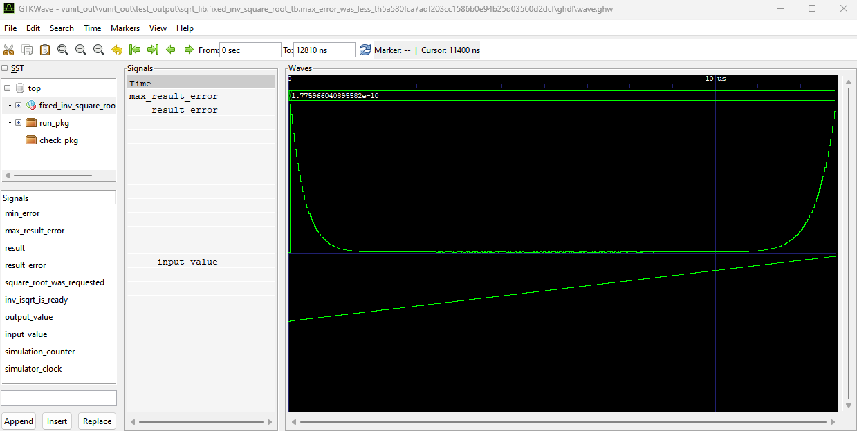
The algorithm is developed in a testbench that can be found here. The algorithm converges if the initial value is close to the real root. As noted before the algorithm converges quadratically, which approximately means that we double the number of correct bits every iteration. This convergence is so fast that for input number between 1.0 and 2.0 a constant initial value is good enough to give roughly 32 bits of accuracy in just 4 iterations. The error behavior with 4 iterations is shown in Fig 1. The error is calculated between the fixed point square root and a reference value that is obtained by counting square root with the real_math library. The figure shows maximum error which with 4 iterations is roughly $1.8\cdot 10^{-10}$.

multiple initial values

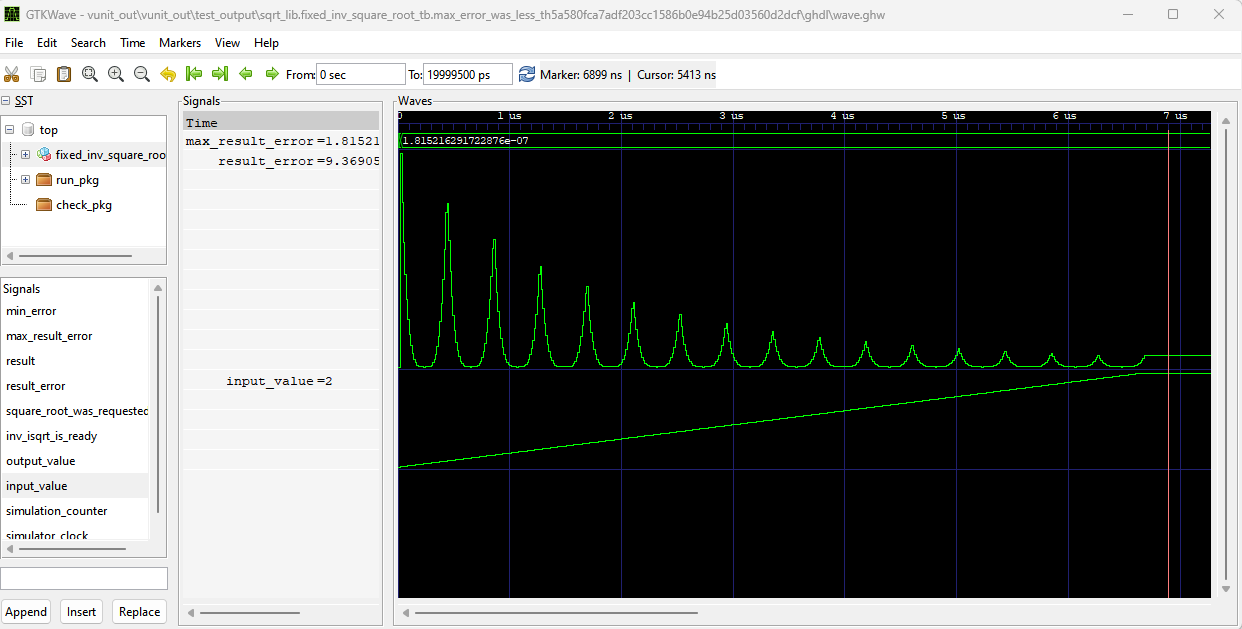
Since the convergence is very fast and the algorithm only requires 3 multiplications of which two can be pipelined, we have an interesting situation with the initial value. There is no benefit obtained from getting a better initial guess unless it is faster to obtain than what it takes to run another iteration. Even a really crude guess gets us fast convergence and the higher accuracy we desire, the higher accuracy initial guess we will need to avoid an iteration through the algorithm. Fig 2. shows the error behavior with the initial value being one of 16 possibilities. This allows us to only use 2 iterations for error less than $2.0\cdot 10^{-7}$ which is close to accuracy of a 32 bit float.

Input range extension beyond $[1.0, 2.0)$

Although having an algorithm that is very accurate for very small range seems limiting, we can extend this range to cover any required range by pre and post scaling. This corresponds with dividing by $2^{(i)}$ until number is between 1.0 and 2.0, then using the NR iteration and lastly post dividing by $2^{(i/2)}$.

With this simple range extension our final inverse square root algorithm has 5 parts. First we scale with factor $2^i$ so that our input number is between 1.0 and 2.0, secondly we get the initial value for NR iterations, third we apply the iteration and lastly we scale the result with $\sqrt{2^i}$ to get the inverse square root and lastly we multiply with the original input number to get its square root.

For example if we want to calculate the square root of 513, we would first scale down the number by $2^{10}$ to get input value to correct range, then apply the inverse square root, then multiply by 513 and lastly scale by $\sqrt{2^{10}}=2^{10/2}$

Square root of 513 :
1. input = 513/2^10 // scale with 2**i
2. x = 0.83 // initial values
3.0 x = 1.5*x - 0.5*input*x*x*x
3.1 x = 1.5*x - 0.5*input*x*x*x
3.2 x = 1.5*x - 0.5*input*x*x*x
4. result = x * 513/2**(10/2)

Range extension in fixed point

Since we are working with bit vectors, the prescaling is a leading zero counter followed by a call to shift_left function. The following function loops thorough the bits of the word and increments a counter when a bit is zero. It resets the counter to zero if one is found. Additionally the function has an argument for maximum depth of the shift in order to allow for restricting the depth of the barrel shifter by breaking down the shift into desired maximum depth.

function get_number_of_leading_zeros
(
    number    : signed;
    max_shift : natural
)
return integer 
is
    variable number_of_leading_zeros : integer := 0;
begin
    for i in integer range number'high-max_shift to number'high loop
        if number(i) = '1' then
            number_of_leading_zeros := 0;
        else
            number_of_leading_zeros := number_of_leading_zeros + 1;
        end if;
    end loop;
    return number_of_leading_zeros;
end get_number_of_leading_zeros;

Full square root algorithm

The complete square root algorithm is implemented using a state machine that sequences the four steps, initial scaling, newton raphson, post multiplication and post scaling. VHDL allows nesting records and procedures, hence the sqrt module is built with the isqrt record and the create_sqrt procedure calls the create_isqrt procedure.

The fixed_sqrt_record holds the shift width of the input scaling, the actual input, its scaled version and a pipeline registers for the barrel shifter.

type fixed_sqrt_record is record
    isqrt                 : isqrt_record;
    shift_width           : natural;
    input                 : fixed;
    scaled_input          : fixed;
    pipeline              : std_logic_vector(2 downto 0);
    multiply_isqrt_result : boolean;
    sqrt_is_ready         : boolean;
end record;

The create_sqrt procedure then combines all of the previous steps into one module. The prescaling is used as the argument to the shift_left function and we also save the shift_width to be used in the post scaling step. Since our post shift is half of the prescaling shift, we need to handle a shift by half a bit in the case that there are odd number of leading zeros. This corresponds with extra multiplication by $\frac{1}{\sqrt{2}}$  in the case the shift width is odd number.

procedure create_sqrt
(
    signal self       : inout fixed_sqrt_record;
    signal multiplier : inout multiplier_record
) is
begin
    create_isqrt(self.isqrt, multiplier);
    self.pipeline     <= self.pipeline(self.pipeline'high-1 downto 0) & '0';
    self.scaled_input <= shift_left(self.input, get_number_of_leading_zeros(self.input)-1);
    self.shift_width  <= get_number_of_leading_zeros(self.input);
    -- get half bit shift in case the number of leading zeros is odd
    if self.shift_width mod 2 = 0 then
        self.post_scaling <= to_fixed(1.0/sqrt(2.0), used_word_length, isqrt_radix);
    else
        self.post_scaling <= to_fixed(1.0, used_word_length, isqrt_radix);
    end if;
    if self.pipeline(self.pipeline'left) = '1' then
        request_isqrt(self.isqrt, self.scaled_input, get_initial_guess(self.scaled_input), self.number_of_iterations);
    end if;
    self.sqrt_is_ready <= false;
    CASE self.state_counter is
        WHEN 0 =>
            if isqrt_is_ready(self.isqrt) then
                multiply(multiplier, get_multiplier_result(multiplier, isqrt_radix), self.post_scaling);
                self.state_counter <= self.state_counter + 1;
            end if;
        WHEN 1 =>
            if multiplier_is_ready(multiplier) then
                multiply(multiplier, get_isqrt_result(self.isqrt), self.input);
                self.state_counter <= self.state_counter + 1;
            end if;
        WHEN 2 =>
            if multiplier_is_ready(multiplier) then
                self.sqrt_is_ready <= true;
                self.state_counter <= self.state_counter + 1;
            end if;
        WHEN others => --do nothing
    end CASE;
end create_sqrt;

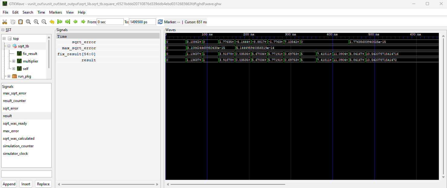
The Full implementation is tested in with a set of numbers that have values between 0.00125 and 511. In the testbench we specify 8 bits for the integer part and we check if the error is less than 1e-7 for the following set of numbers

 
constant input_values : real_array := (1.291356  , 1.0       , 15.35689       ,
                                       0.00125   , 32.153    , 33.315         ,
                                       0.4865513 , 25.00     , 55.02837520    ,
                                       122.999   , 34.125116 , 111.135423642);

The sqrt algorithm in the testbench runs through the iteration 5 times and we can see that the maximum error of the caluclation is less than 6e-14 meaning that it is close to the accuracy offered by the 64 bit float of the real datatype.

Hardware test

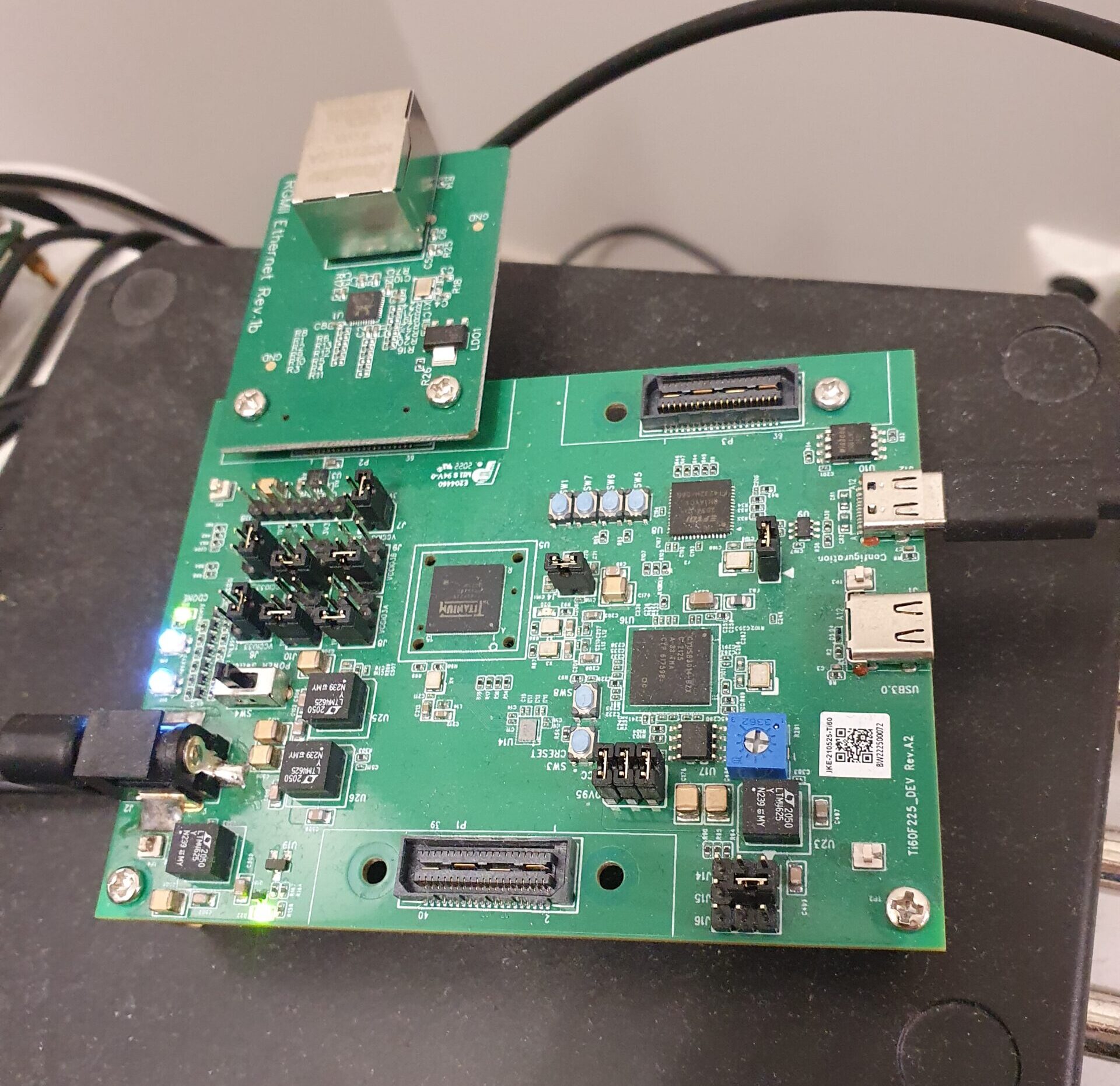
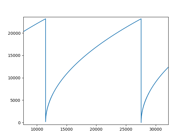
We test the square root algorithm synthesis with Efinix Titanium evaluation kit and the test project is available in the github. The project also has compile scripts for Vivado, Quartus and Lattice Diamond hence you can test it with any of the toolchains. The test project communicates with the fpga using uart which is mapped to the internal bus of the fpga. We run numbers 0 to 65535 through the algorithm which is implemented in 18 bit word length. The result of this can be seen in Fig 5.

We create a test_sqrt entity which has an entity which maps the result to internal bus which allows it to be read from uart.

entity test_sqrt is
    port (
        clk                      : in std_logic;
        input_number             : in integer range 0 to 2**16-1;
        request_sqrt_calculation : in boolean;
        bus_in                   : in fpga_interconnect_record;
        bus_out                  : out fpga_interconnect_record
    );
end entity test_sqrt;
architecture rtl of test_sqrt is
    signal multiplier : multiplier_record := init_multiplier;
    signal sqrt : fixed_sqrt_record := init_sqrt;
    signal result : signed(17 downto 0) := (others => '0');
begin
    test : process(clk)
    begin
        if rising_edge(clk) then
            create_multiplier(multiplier);
            create_sqrt(sqrt,multiplier);
            init_bus(bus_out);
            connect_read_only_data_to_address(
                bus_in  => bus_in,
                bus_out => bus_out,
                address => 15357,
                data    => to_integer(result));
            if request_sqrt_calculation then
                request_sqrt(sqrt, to_signed(input_number, 18));
            end if;
            if sqrt_is_ready(sqrt) then
                result <= get_sqrt_result(sqrt, multiplier, 15);
            end if;
        end if; --rising_edge
    end process test;    
end rtl;

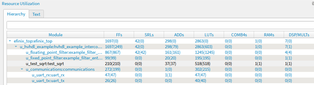
The resource usage of the square root with the efinix titanium is shown in Fig. 6. The Efinity synthesizes the lookup table to ram hence it uses a single ram block as well as the multiplier. The example design uses 18x18 bit multiplier and it takes roughly 520 luts as well as one multiplier and one ram block. The design also has maximum clock rate at slightly over 200Mhz.

Final notes

The square root presented here allows calculating square root of a fixed point number. The design has some substantial speedups that are not yet implemented. The output barrel shifter fetches the result directly from the multiplier register and the input shift is done with a purely combinatorial design. Both of these could be done with a single shifter that limits the shift depth. Using a single shift hardware for both input and output would reduce the resource usage and it would also get much better timing. Though it is not an issue with the titanium, building the same design with Efinix Trion does struggle to meet timing at 120MHz. The output radix is still dependent on the input radix which makes the use of this algorithm slightly more inconvenient than necessary. The initial value choise also maps into a ram though without some necessary input and output registers which makes it quite slow.

The lookup table also is full word width, though it is definetly not necessary to do so. Even a very crude initial value would yield rougly the same peak error since the erro values close to 1.0 are much greater than the rest of the range. The fixed point library is a continuously developed and I will be implementing all of these fixes at some point.

Sign in