


Fluxions for Fun and Profit: Euler, Trapezoidal, Verlet, or Runge-Kutta?
Today we're going to take another diversion from embedded systems, and into the world of differential equations, modeling, and computer simulation.
DON'T PANIC!
First of all, just pretend I didn't bring up anything complicated. We're exposed to the effects of differential equations every day, whether we realize it or not. Your car speedometer and odometer are related by a differential equation, and whether you like math or not, you probably have some comprehension of what's going on: you press the accelerator, the car accelerates, the speedometer goes up, the odometer counts up faster.
If at any time you feel anxious about math when reading this blog, just skip the equations you're reading and move on.
And to address any of you who are thinking "I just want to mess around with microcontrollers and Arduino, WTF does this have to do with me?", I'll just say that we'll use some results from this discussion in future blogs.
OK, ready?
Horseshoes, Hand Grenades, and Computer Simulation: Getting Close Enough
Let's look at a really simple example, a metal bead sliding on a horizontal rod dipped in water. We need a way to model it. If you're familiar with physics, perhaps you'll remember the following equations, where t is time; \( \frac{d}{dt} \) is the time derivative, or rate of change with time; x is the position of the metal bead; v is the velocity; m is the mass of the bead; F is the force on the bead, and k is a constant that represents the resistance of the water to motion:
$$\begin{eqnarray} m\frac{dv}{dt} & = & F = -kv \cr \frac{dx}{dt} & = & v \end{eqnarray}$$
Again, don't panic! Let's calculate \( \tau = m/k \) and we can reduce this to
$$\begin{eqnarray} \frac{dv}{dt} & = & -\frac{1}{\tau} v \cr \frac{dx}{dt} & = & v \end{eqnarray}$$
The general solution to these equations is
$$ \begin{eqnarray} v &=& v_0 e^{-t/\tau} \cr x &=& x_0 + v_0\tau(1-e^{-t/\tau}) \end{eqnarray}$$
for arbitrary constants \( v_0 \) and \( x_0 \) which represent the initial velocity and position of the bead. If we graph them, they look like this:
import numpy as np
import matplotlib.pyplot as plt

tstart = 0
tend = 4
t_exact = np.arange(tstart,tend,0.001)
v0 = 3
x0 = 2
tau = 0.5
def fv(t):
    return v0*np.exp(-t/tau)
def fx(t):
    return v0*tau*(1-np.exp(-t/tau)) + x0
v_exact = fv(t_exact)
x_exact = fx(t_exact)

def interleave_timeseries(tlist,xlist):
    args = []
    t = iter(tlist)
    for x in xlist:
        if isinstance(x,basestring):
            args.append(x)
        else:
            args.append(t.next())
            args.append(x)
    return args

def plot_vx(tlist,vlist,xlist):
    fig=plt.figure()
    ax=fig.add_subplot(2,1,1)
    ax.plot(*interleave_timeseries(tlist,vlist))
    ax.set_ylabel('v')

    ax=fig.add_subplot(2,1,2)
    ax.plot(*interleave_timeseries(tlist,xlist))
    ax.set_xlabel('t')
    ax.set_ylabel('x')
    return fig

plot_vx([t_exact],[v_exact],[x_exact]);

This is an example of an exact solution of a differential equation. How to solve differential equations exactly is beyond the scope of this article, and for most realistic differential equations it's either impossible or painful. If you want to learn more, go take a differential equations course. More power to you.
The rest of us will talk about using numerical methods to get an approximate solution to differential equations. The problem here is the following:
Suppose your best friend Ed comes up to you with some equations that look like:
$$\begin{eqnarray} \frac{dx_0}{dt} &=& f_0(t,x_0,x_1,...) \cr \frac{dx_1}{dt} &=& f_1(t,x_0,x_1,...) \cr \frac{dx_2}{dt} &=& f_2(t,x_0,x_1,...) \cr \frac{dx_3}{dt} &=& f_3(t,x_0,x_1,...) \cr ... \end{eqnarray}$$
where the x's are some unknown waveforms, and the f's are functions Ed gives to you. He wants you to help him solve these equations for numerically. First of all, don't hit Ed. He's actually done the hard part; most of the time the hard work is just coming up with what equations to solve, and putting them in a standard form like this. Second of all, forget this \( \frac{d}{dt} \) stuff. Isaac Newton and Gottfried Leibniz went through the hard part in the late 1600's, and now we're cursed with calculus, and what Newton called fluxions. Newton didn't use this \( \frac{d}{dt} \) stuff; instead of the \( \frac{dx}{dt} \) that Leibniz used, Newton wrote \( \dot{x} \). But we don't want to use that either; we just want it to go away, because it involves infinitesimal mathematics, which we don't want to deal with, since they're the equivalent of moving large piles of sand one grain at a time, only with smaller bits. So let's see some techniques for approximating the solution of differential equations.
Euler integration
Euler integration is easy; anytime you see \( \frac{d}{dt} \) you just replace it with \( \frac{\Delta}{\Delta t} \) to convert the differential equations into difference equations, which basically just tell you how to figure out what happens next (at time \( t+\Delta t \)) from what's happening now (at time \( t \)).
Let's look at our bead-on-a-rod example:
$$\begin{eqnarray} \frac{dv}{dt} & = & -\frac{1}{\tau} v \cr \frac{dx}{dt} & = & v \end{eqnarray}$$
We make the switch from \( d \) to \( \Delta \) and multiply the right hand side by \( \Delta t \):
$$\begin{eqnarray} \Delta v & = & -\frac{1}{\tau} v \Delta t \cr \Delta x & = & v \Delta t \end{eqnarray}$$
In pseudocode this will look like
 // setup initial conditions
 v = v0
 x = x0
 t = t0
 while (t < t1):
   v_next = v + (-1/tau) * v * dt
   x_next = x + v * dt

   t += dt
   v = v_next
   x = x_next
And let's go ahead and do it:
fderiv = lambda t,v,x: (-1/tau*v,v)
def testEuler(tstart,tend,fderiv,dt):
  v = v0
  x = x0
  vapprox = [v]
  xapprox = [x]

  tapprox = [tstart]
  for t in np.arange(tstart+dt,tend+dt,dt):
    dvdt,dxdt = fderiv(t,v,x)
    v_next = v + dvdt * dt
    x_next = x + dxdt * dt

    v = v_next
    x = x_next
    tapprox.append(t)
    vapprox.append(v)
    xapprox.append(x)

  return (np.array(tapprox), np.array(vapprox), np.array(xapprox))

(tapprox,vapprox,xapprox) = testEuler(tstart, tend, fderiv, 0.25)
plot_vx([t_exact, tapprox], [v_exact, vapprox,'.'], [x_exact, xapprox,'.']);
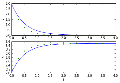
Well, that's okay. Not great, but okay. How did we pick the value for dt, though? If we make it smaller, it works better, and if we make it too large, it doesn't work very well at all:
(tapprox,vapprox,xapprox) = testEuler(tstart, tend, fderiv, 0.1)
plot_vx([t_exact, tapprox], [v_exact, vapprox,'.'], [x_exact, xapprox,'.']);

(tapprox,vapprox,xapprox) = testEuler(tstart, tend, fderiv, 0.6)
plot_vx([t_exact, tapprox], [v_exact, vapprox,'.'], [x_exact, xapprox,'.'])
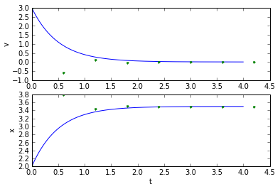

In this specific case, the timestep needs to be faster than the system time constant \( \tau = 0.5 \) seconds. That's true in general with Euler integration: the simulation timestep needs to be faster than the fastest dynamic of the system. (For those of you more familiar with the math, the technical aspect of this for linear differential equations, is that if you put the equation in matrix form e.g. \( \frac{dx}{dt}=Ax \), then for each eigenvalue λ of the matrix A, the product of the timestep and the real part of λ should be less than 1.)
How fast does the timestep need to be for Euler integration (or any other method, for that matter) to achieve a given accuracy? In general this is a hard problem; variable timestep methods attempt to choose a timestep at runtime based on a given output tolerance, and I'm not even going to attempt to dig into that math. If you use Simulink for continuous systems, you're probably working with a variable timestep solver.
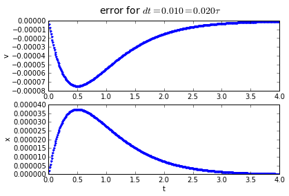
Let's look at the error. Remember, I went on a rant last time about how graphs of close comparisons should always show the error, so I'll walk the walk, not just talk the talk.
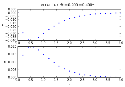
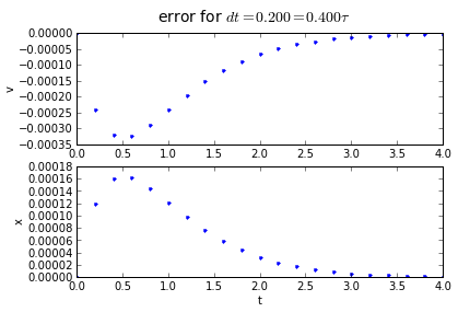
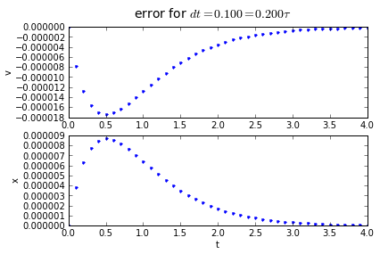
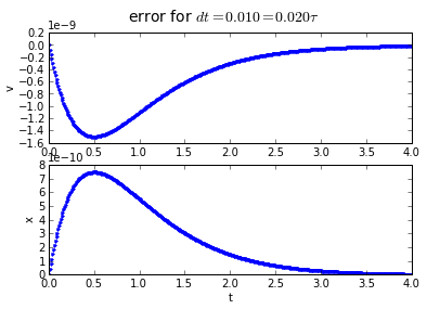
for dt in [0.2, 0.1, 0.01]:
    (tapprox,vapprox,xapprox) = testEuler(tstart, tend, fderiv,dt)
    fig = plot_vx([tapprox],[fv(tapprox)-vapprox,'.'],[fx(tapprox)-xapprox,'.'])
    fig.suptitle('error for $dt = %.3f = %.3f\\tau $' % (dt, dt/tau),fontsize=14)
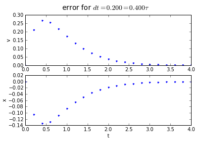
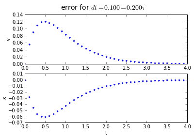
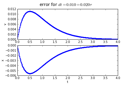
You'll note that the error is proportional to the timestep: If we want to make the error 10 times smaller, we need to make the timestep 10 times smaller.
If you don't need high accuracy, Euler integration is often good enough, and use a timestep between 1/5 and 1/10 of the fastest system time constant. If you do need high accuracy, consider using one of the methods discussed later. Many systems don't need high accuracy, for example, if you're programming game physics, or you just need a rough approximation of your real system (often the coefficients of your equation are only approximate anyway, so there's no sense in being super-accurate in simulating a system where you only know the coefficients with 5% accuracy).
Trapezoidal integration: the next step
Euler integration is a predictive method that assumes things change linearly over a small period of time. Remember, we determine what's going to happen over the next timestep based on what's happening right now, and we totally ignore any changes that happen during the timestep. Let's look at our example more closely for timestep 0.25:
dt = 0.25
plt.plot(t_exact,v_exact,[0,dt],[v0, v0-1/tau*v0*dt],'.:')
plt.xlim(0,0.3001); plt.ylim(1.4,3);
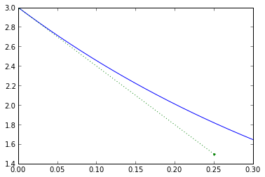
Everything starts out nicely, but the real system doesn't change linearly with time, so during the timestep we accumulate errors.
There's also a similar algorithm which is called Backward Euler integration (the simple Euler integration is a Forward Euler integration), which uses the value of \( \frac{dx}{dt} \) at the end of the timestep. But we don't know this value at the beginning of the timestep, so instead we get an equation that we have to solve each timestep to determine what to do. Fortunately this equation is simpler than the original differential equation.
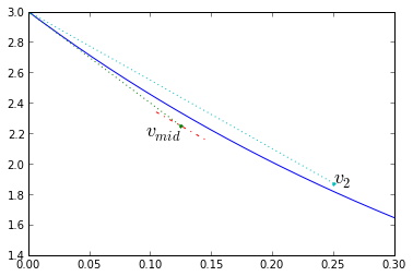
Trapezoidal integration is a predictive/corrective method to solve \( \frac{dx}{dt} = f(t,x) \). We start with Euler integration, using the slope at the beginning of the timestep \( k_1 = f(t_1,x_1) \), to compute a first approximation for the end of timestep \( x _ {2a} = x(t_1) + k_1 \Delta t \). Then calculate a new slope at that endpoint \( k_2 = f(t_2,x_2) \), and use the average \( \frac{k_1+k_2}{2} \) as the "real" slope during that timestep, so that \( x_2 = x_1 + \frac{k_1+k_2}{2}\Delta t \).
dt = 0.25
v1 = v0; t1 = 0; t2 = t1+dt
k1,_ = fderiv(t1,v1,0)   # ignore the 2nd variable
v2a = v1 + dt*k1        # initial projection
k2,_ = fderiv(t2,v2a,0)
v2 = v1 + dt*(k1+k2)/2
# correction based on average of initial, final slopes of the initial approximation
a=0.08
plt.plot(t_exact,v_exact,[t1,t2],[v1, v2a],'.:')
plt.plot([t2-dt*a,t2+dt*a],[v2a-k2*dt*a,v2a+k2*dt*a],'-.')
plt.plot([t1,t2],[v1,v2],'.:')
plt.text(t2,v2a,'$v_{2a}$',fontsize=18)
plt.text(t2,v2,'$v_{2}$',fontsize=18)
plt.xlim(0,0.3001); plt.ylim(1.4,3);
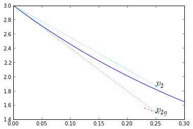
Note how the corrected timestep is much more accurate. Let's try trapezoidal integration on our system with various timesteps, and look at the error:
def testTrapz(tstart,tend,fderiv,dt):
v = v0
x = x0
vapprox = [v]
xapprox = [x]
tapprox = [tstart]
for t in np.arange(tstart+dt,tend+dt,dt):
kv1,kx1 = fderiv(t,v,x)
v_2a = v + kv1 * dt
x_2a = x + kx1 * dt
kv2,kx2 = fderiv(t,v_2a,x_2a)
v_next = v + (kv1+kv2)/2*dt
x_next = x + (kx1+kx2)/2*dt
v = v_next
x = x_next
tapprox.append(t)
vapprox.append(v)
xapprox.append(x)
return (np.array(tapprox), np.array(vapprox), np.array(xapprox))
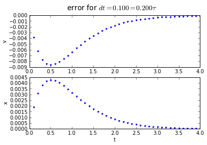
for dt in [0.2, 0.1, 0.01]:
(tapprox,vapprox,xapprox) = testTrapz(tstart, tend, fderiv, dt)
fig = plot_vx([tapprox],[fv(tapprox)-vapprox,'.'],[fx(tapprox)-xapprox,'.'])
fig.suptitle('error for $dt = %.3f = %.3f\\tau $' % (dt, dt/tau),fontsize=14)

Trapezoidal integration has an error that is proportional to the square of the timestep: if we divide the timestep by 10, we divide the error by 100. Hurray!
The Midpoint Method
There's another method which is very similar to trapezoidal integration. In trapezoidal integration we used a trial timestep to get to the end of the timestep, then used a slope that was the average of the beginning and end slopes of the trial timestep. In the midpoint method, we use a trial timestep to get to the middle of the timestep, and use the slope found there to improve the estimate of the whole timestep. More precisely: We start with Euler integration, using the slope at the beginning of the timestep \( k_1 = f(t_1,x_1) \), to compute a first approximation for the middle of the timestep \( x _ {mid} = x(t_1) + k_1 \frac{\Delta t}{2} \). Then calculate a new slope at that midpoint \( k_2 = f(t_1 + \frac{\Delta t}{2},x _ {mid}) \), and use it as the "real" slope during the timestep, so that \( x_2 = x_1 + k_2\Delta t \).
dt = 0.25
v1 = v0; t1 = 0; t2 = t1+dt; tmid = t1+dt/2
k1,_ = fderiv(t1,v1,0)  # ignore x-component
vmid = v1 + dt*k1/2        # projection to midpoint
k2,_ = fderiv(tmid,vmid,0)
v2 = v1 + dt*k2
# slope based on midpoint derived from initial approximation
a=0.08
plt.plot(t_exact,v_exact,[t1,tmid],[v1, vmid],'.:')
plt.plot([tmid-dt*a,tmid+dt*a],[vmid-k2*dt*a,vmid+k2*dt*a],'-.')
plt.plot([t1,t2],[v1,v2],'.:')
plt.text(tmid,vmid,'$v_{mid}$',fontsize=18,horizontalalignment='right',
        verticalalignment='top')
plt.text(t2,v2,'$v_{2}$',fontsize=18)
plt.xlim(0,0.3001); plt.ylim(1.4,3);
Again, let's look at the error:
def testMidpoint(tstart,tend,fderiv,dt):
  v = v0
  x = x0
  vapprox = [v]
  xapprox = [x]

  tapprox = [tstart]
  for t in np.arange(tstart+dt,tend+dt,dt):
    kv1,kx1 = fderiv(t,v,x)
    v_mid = v + kv1 * dt/2
    x_mid = x + kx1 * dt/2
    t_mid = t + dt/2

    kv2,kx2 = fderiv(t_mid,v_mid,x_mid)
    v_next = v + kv2*dt
    x_next = x + kx2*dt

    v = v_next
    x = x_next
    tapprox.append(t)
    vapprox.append(v)
    xapprox.append(x)

  return (np.array(tapprox), np.array(vapprox), np.array(xapprox))

for dt in [0.2,0.1, 0.01]:
    (tapprox,vapprox,xapprox) = testMidpoint(tstart, tend, fderiv, dt)
    fig = plot_vx([tapprox],[fv(tapprox)-vapprox,'.'],[fx(tapprox)-xapprox,'.'])
    fig.suptitle('error for $dt = %.3f = %.3f\\tau $' % (dt, dt/tau),fontsize=14)


The error behavior is almost exactly the same as the trapezoidal method. There is one aspect of the midpoint method which is better: if you have a problem which has a sharp curve in its slope, or you are getting close to a discontinuity, the midpoint method is more "cautious": it only probes a half-step ahead to get its predicted result, whereas the trapezoidal method probes a full step ahead.
Runge-Kutta
Okay, so there were these two German guys, Carl Runge and Martin Kutta... along with a 3rd German guy named Karl Heun who missed out on getting the credit. In 1895 Runge published a numerical technique for solving differential equations; Heun improved it a few years later, and Kutta improved it further for his Ph.D. thesis. These were pioneers in the modern field of numerical methods; I wonder how it was seen back then — apparently Runge got looked down upon by both mathematicians and physicists for fooling around in this middle ground of "applied mathematics".
In any case, the Runge-Kutta(-Heun) technique is a method of increasing the accuracy of solving differential equations using several trial integration steps. The method itself is parameterized, but Runge-Kutta usually refers to a 4th-order method, which is calculated as follows:
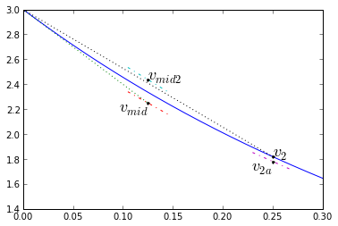
$$\begin{eqnarray} k_1 &=& f(t_1,x_1) & \text{[Compute initial slope]} \cr k_2 &=& f(t_1+\frac{\Delta t}{2},x_1+k_1\frac{\Delta t}{2}) & \text{[Compute slope at midpoint, assuming initial slope k1]} \cr k_3 &=& f(t_1+\frac{\Delta t}{2},x_1+k_2\frac{\Delta t}{2}) & \text{[Compute slope at midpoint, assuming initial slope k2]} \cr k_4 &=& f(t_1+\Delta t,x_1+k_3\Delta t) & \text{[Compute slope at end, assuming initial slope k3]} \cr x_2 &=& x_1 + \frac{k_1+2k_2+2k_3+k_4}{6}\Delta t & \text{[Now compute end value based on a weighted average of slopes]} \end{eqnarray}$$
The slope diagram looks like this:
dt = 0.25
v1 = v0; t1 = 0; t2 = t1+dt; tmid = t1+dt/2
k1,_ = fderiv(t1,v1,0)  # ignore x-component
vmid = v1 + dt*k1/2        # projection to midpoint
k2,_ = fderiv(tmid,vmid,0)
vmid2 = v1 + dt*k2/2       # 2nd projection to midpoint
k3,_ = fderiv(tmid,vmid2,0)
v2a = v1 + dt*k3       # projection to end
k4,_ = fderiv(t2,v2a,0)
v2 = v1 + dt*(k1+2*k2+2*k3+k4)/6       # final answer!

# slope based on midpoint derived from initial approximation
a=0.08
plt.plot(t_exact,v_exact,[tmid],[vmid],'.k',[t1,tmid],[v1,vmid],':')
plt.plot([tmid-dt*a,tmid+dt*a],[vmid-k2*dt*a,vmid+k2*dt*a],'-.')
plt.plot([tmid-dt*a,tmid+dt*a],[vmid2-k3*dt*a,vmid2+k3*dt*a],'-.')
plt.plot([t2-dt*a,t2+dt*a],[v2a-k4*dt*a,v2a+k4*dt*a],'-.')
plt.plot([tmid],[vmid2],'.k',[t2],[v2a],'.k',[t1,t2],[v1,v2],'.k:')
plt.text(tmid,vmid,'$v_{mid}$',fontsize=18,horizontalalignment='right',
        verticalalignment='top')
plt.text(tmid,vmid2,'$v_{mid2}$',fontsize=18)
plt.text(t2,v2a,'$v_{2a}$',fontsize=18,horizontalalignment='right',
        verticalalignment='top')
plt.text(t2,v2,'$v_{2}$',fontsize=18)
plt.xlim(0,0.3001); plt.ylim(1.4,3);
And the error behavior:
def testRK4(tstart,tend,fderiv,dt):
  v = v0
  x = x0
  vapprox = [v]
  xapprox = [x]

  tapprox = [tstart]
  for t in np.arange(tstart+dt,tend+dt,dt):
    kv1,kx1 = fderiv(t,v,x)
    v_mid = v + kv1 * dt/2
    x_mid = x + kx1 * dt/2
    t_mid = t + dt/2

    kv2,kx2 = fderiv(t_mid,v_mid,x_mid)
    v_mid2 = v + kv2*dt/2
    x_mid2 = x + kx2*dt/2

    kv3,kx3 = fderiv(t_mid,v_mid2,x_mid2)
    v_end1 = v + kv3*dt
    x_end1 = x + kx3*dt

    kv4,kx4 = fderiv(t + dt,v_end1,x_end1)
    v_next = v + (kv1+2*kv2+2*kv3+kv4)/6*dt
    x_next = x + (kx1+2*kx2+2*kx3+kx4)/6*dt

    v = v_next
    x = x_next
    tapprox.append(t)
    vapprox.append(v)
    xapprox.append(x)

  return (np.array(tapprox), np.array(vapprox), np.array(xapprox))

for dt in [0.2,0.1, 0.01]:
    (tapprox,vapprox,xapprox) = testRK4(tstart, tend, fderiv, dt)
    fig = plot_vx([tapprox],[fv(tapprox)-vapprox,'.'],[fx(tapprox)-xapprox,'.'])
    fig.suptitle('error for $dt = %.3f = %.3f\\tau $' % (dt, dt/tau),fontsize=14)
4th order Runge-Kutta integration has an accumulated error that is proportional to the 4th power of the timestep: if we divide the timestep by 10, we divide the error by 10000. Quadruple-hurray!
Symplectic integration methods
Numerical methods for differential equations is a huge subject, and there's a lot more than just pointing out a few methods. Other techniques are available and include variable-step methods, and methods that deal well with "stiff" differential equations where the behavior changes very rapidly with operating point around a particular boundary, and requires a very small timestep near that boundary. I won't be getting into these details.
I would like to briefly cover a few specialized methods for so-called symplectic integration problems, where the system state can be defined in terms of energy that can be divided up into separable components, which are subject to some kind of conservation-of-energy law. Many physics and electromechanical systems fall into this category. Don't ask me to clarify further; I never studied Hamiltonian systems in college and my eyes kind of glaze over when I look at the equations.
But one important type of equation that is easy to recognize, and falls into this category, is when you have a set of equations for velocity/position/acceleration that have this type of structure:
$$\begin{eqnarray} \frac{dv}{dt} &=& a(v,x,t) \cr \frac{dx}{dt} &=& v \end{eqnarray}$$
The system state is composed of velocity v and position x; position is dictated completely by velocity (the 2nd equation above). Often you are dealing with gravity or springs or pendulums where energy is conserved. In these sorts of equations the acceleration can usually be separated into a term that is a function of x alone (covering transfer of potential energy), plus terms that represents damping or drag or an external force acting on an object.
For these sorts of physical systems there are methods that take advantage of the idea of conservation of energy: they are designed so that some of the error terms cancel out when used on physical systems. Runge-Kutta is not one of these methods; it's a very good general method, but if you use it on a physical system and look at the total energy, it may drift up or down over time. (The other methods discussed above — Euler, trapezoidal, and midpoint — suffer from energy drift as well.)
Semi-implicit Euler integration
Let's look at our basic Euler approach again, applied to the mechanical equations of our system:
v2 = v1 + a(v1,x1,t1) * dt
x2 = x1 + v1 * dt
Now we'll make one little bitty change here:
v2 = v1 + a(v1,x1,t1) * dt
x2 = x1 + v2 * dt
Did you spot the change? The regular Euler approach computes new position and velocity as a function of old position and velocity. Our tweaked approach computes the velocity update the same way, but then uses this new velocity update to compute the position. This is called the semi-implicit Euler method and it is much more stable for solving Hamiltonian systems.
Verlet integration
You'll like Verlet integration. It's simple and involves only 1 derivative evaluation per timestep (vs. 2 for trapezoidal/midpoint and 4 for Runge-Kutta). The basic idea of the so-called Position Verlet and Velocity Verlet methods is that you split the timestep in half, and then interleave the position and velocity calculations.
Given a starting system state v1, x1 at time t1, we can calculate the system state at time t2 = t1 + dt as follows.
For Velocity Verlet:
a1 = a(x1,t1)
v_mid = v1 + a1 * dt/2
// Requires that acceleration doesn't depend on velocity,
// in which case we can use acceleration calculation saved from last time

x2 = x1 + v_mid * dt
a2 = a(x2,t1+dt)
// save this for next time
v2 = vmid + a2 * dt/2
Alternatively, you can use this form:
a1 = a(x1,t1)
x2 = x1 + v1*dt + a1*dt*dt/2
a2 = a(x2,t1+dt)
v2 = v1 + (a1+a2)*dt/2
For Position Verlet:
x_mid = x1 + v1 * dt/2
v2 = v1 + a(x_mid, t1 + dt/2) * dt
x2 = x_mid + v2 * dt/2
That's it! If the acceleration depends a little bit on velocity (e.g. viscous damping), it's probably OK to use the Verlet methods, but you'll need to accept one or more of the following:
- accuracy is going to be degraded if the velocity-dependent term is not small
- you may need to add a correction term to first calculate a coarse estimate of velocity at the time that acceleration is calculated: at end of the timestep for Velocity Verlet, and at the middle of the timestep for Position Verlet
- for Velocity Verlet the acceleration calculation can't be reused at the beginning of the next timestep, since the velocity used for that calculation is not up to date.
In these cases I would probably pick the Position Verlet method, as it appears as though the error would be smaller if you just use 1 acceleration calculation, but I don't have any theoretical basis or evidence to back up my intuition.
Higher-order methods
Just as we have Euler, trapezoidal, and Runge-Kutta for a sequence of increasingly-complicated and increasingly-accurate techniques for general differential equations, there are higher-order methods for symplectic integrators. One of these was discovered in the 1980s by Forest and Ruth, which uses this interleaved algorithm:
K = 1/(2 - cube_root(2)) = 1.3512071919596578....
x1a = x1  + v1 * K/2 * dt
v1a = v1  + a(x1a) * K * dt
x1b = x1a + v1a * (1-K)/2 * dt
v1b = v1a + a(x1b) * (1-2*K) * dt
x1c = x1b + v1b * (1-K)/2 * dt
v2  = v1b + a(x1c) * K * dt
x2  = x1c + v2 * K/2 * dt
for a total of 3 evaluations of acceleration needed.
Comparing apples to apples: how to pick an equation solver
We've seen a bunch of techniques, but how are you supposed to know which one to pick?
First of all, make sure you are comparing apples to apples. Don't forget how many function evaluations it takes, namely the number of times you have to calculate the right side of your differential equations (i.e. acceleration above). In many cases this comprises the bulk of the CPU time needed. Runge-Kutta is almost always better than trapezoidal or Euler, but please note that it takes 4 function evaluations, whereas trapezoidal and midpoint take 2, and Euler takes 1. That being said, Runge-Kutta is still a better choice in many cases. If I had to budget CPU time for 1000 calculations per second, I would rather use 250 Runge-Kutta iterations per second than 500 midpoint or trapezoidal iterations, and any of them over 1000 Euler iterations per second.
These solvers are also generally easy enough to try out and see for yourself which works well in your application. I would definitely keep your code modular: try to make it so that the solver code and the differential equation function are separate, so that you can swap out solvers easily without having to revalidate your differential equation calculations.
If you have a system which fits well into Verlet or Forest-Ruth methods, use them instead of Runge-Kutta, since it will increase the accuracy relative to the number of function evaluations, and will also do a better job with conservation of energy.
Finally there are plenty of cases where lower-order solvers (Euler) are still often the best choice because of their simplicity. In particular:
- if you are working with a highly unpredictable input term coming from a sampled data system
- if you are working on a system where the coefficients are not precisely known
- if you are working on a system where the dynamics are not precisely known (e.g. small nonlinearities)
In these cases, the effect of input/system uncertainty often dominates any numerical errors, and there's not much point in being ultraprecise with an equation solver if it's a very minor contribution to overall system error.
The Differential Equation Solver Shootout
Two simple examples of differential equations are a rigid pendulum and an orbiting satellite. Both are nonlinear but well-understood.
Orbiting satellite (Kepler's problem)
Here we have a small satellite, and a single large planet/star. The equations of motion are:
$$\begin{eqnarray} \frac{d\vec{r}}{dt} &=& \vec{v} \cr \frac{d\vec{v}}{dt} &=& -\frac{MG\vec{r}}{|\vec{r}|^3}
\end{eqnarray}$$
where \( \vec{r} \) is the position vector of the satellite relative to the planet, \( \vec{v} \) is the velocity vector of the satellite, M is the mass of the planet, and G is the gravitational constant.
The solution of these equations is a fixed orbit which is a conic section (circle/ellipse/parabola/hyperbola) with a center/focus at the center of the planet, and it's been well-understood for about 400 years.
When I was researching this article, there was already a comparison online of the different methods using Kepler's problem as a test case. But it claims Runge-Kutta performs poorly, and that was a red flag for me — either the author's implementation of it has an error, or the timestep is so low that it's not a useful comparison. In any case, I set out to create a good test case for evaluating the different solvers with Kepler's problem.
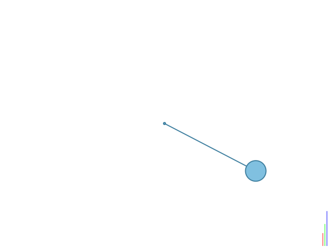
You can try out my example by clicking on the image below. (If I can figure out how to embed it directly in this article, I will do so.)
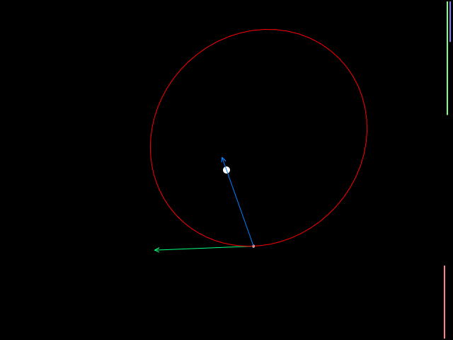
Here you can watch a satellite in orbit, and select from the 8 solvers we discussed here. The simulation also reports a number of parameters. The first two, radius (= distance from the planet's center) and velocity, change with time. The rest of them (min/max radius, period, angular momentum, eccentricity, and total energy) are constant for a satellite that undergoes acceleration from only the planet's gravity. You can alter the orbit by clicking on the diagram and then using the arrow keys to add thrust.
The arrows pointing from the satellite denote its velocity (green), its gravitational acceleration (blue), and acceleration from thrust (yellow). The bars on the right side of the simulation diagram show changing kinetic energy (orange, \( KE = \frac{1}{2}mv^2 \)), potential energy (green, \( PE = \frac{-GMm}{r} \)), and total energy (blue, \( KE+PE \)).
Orbital dynamics are kind of nonintuitive: if you add reverse thrust to slow a satellite down, its radius decreases and it actually speeds up; if you add thrust to speed it up, its radius increases and it slows down. Have fun playing around!
Anyway, the plain Euler solver is lousy, experiencing drifts in orbital parameters even at 1500 calculations per second. The other solvers are generally pretty good except for tight orbits; Runge-Kutta and Forest-Ruth show barely any parameter drift, even at lower calculation rates. The four symplectic integrators (implicit Euler, the two Verlet integrators, and Forest-Ruth) have the property that the angular momentum doesn't drift at all, and even though the remaining orbital parameters may change over time, they change periodically rather than cause the satellite to drift off to infinity or crash into the planet. Forest-Ruth is the champion here; it works well even at very low update rates. Runge-Kutta is pretty good but it experiences orbital decay.
Rigid pendulum
This one's simpler. The state equations of a rigid pendulum are
$$\begin{eqnarray} \frac{d\theta}{dt} &=& \omega \\ \frac{d\omega}{dt} &=& -\frac{g}{L} \sin \theta - B \omega \end{eqnarray}$$
where θ is the angle of the pendulum relative to the bottom of its swing, ω is its angular velocity, g = the gravitational acceleration (9.8m/s2 at sea level on Earth), L is the pendulum length, and B is a damping coefficient.
Click on the drawing below to play around with it. :-)
At low damping coefficients, you can see whether the solver preserves energy or not. The plain Euler method incorrectly increases total energy; trapezoidal, midpoint, and Runge-Kutta decrease the total energy; the symplectic methods produce small oscillations of total energy. Again, Runge-Kutta and Forest-Ruth are the most accurate of the solvers shown here.
Summary
Differential equations are a pain to solve, but if you have a computer there are plenty of methods to solve them numerically. I've presented several of them here, both for general differential equations, and equations of Hamiltonian systems involving exchange of energy between speed and position. The Hamiltonian systems can use symplectic integrators as solvers, which take advantage of the structure of these systems to conserve total energy and reduce the number of function evaluations for a given accuracy. Runge-Kutta is a widely-used fourth-order method for solving equations in general.
If you have systems with lots of uncertainties (and embedded systems that must estimate the state of physical system usually fall into this category), the simple 1st-order Euler method is usually adequate. If not, try one of the other solvers presented here.
Timestep determines the numerical error of a simulation; reducing the timestep reduces the error. Please note that a reduced timestep also places more stringent demands on numerical resolution: smaller timesteps mean that you need more numerical precision in your system state.
Happy equation-solving! Next time we'll get back to a much more concrete topic of circuit design.
References
Numerical Methods for Differential Equations, Brian Storey, Olin College of Engineering.
Who invented the great numerical algorithms?, Nick Trefethen, Oxford Mathematical Institute.
The Störmer-Verlet Method, F. Crivelli, Swiss Federal Institute of Technology, Zurich.
The leapfrog method and other "symplectic" algorithms for integrating Newton's laws of motion, Peter Young, University of California at Santa Cruz. This is a really good writeup of the symplectic integrators; in fact, it's the only easy-to-read reference on Forest-Ruth that I was able to find.
© 2013 Jason M. Sachs, all rights reserved.
Stay tuned for a link to this code in an IPython Notebook. I'll put it up on the web, and I do plan to release this in an open-source license, I just have to do a little more homework before I pick the right one.


- Comments
- Write a Comment Select to add a comment

To post reply to a comment, click on the 'reply' button attached to each comment. To post a new comment (not a reply to a comment) check out the 'Write a Comment' tab at the top of the comments.
Please login (on the right) if you already have an account on this platform.
Otherwise, please use this form to register (free) an join one of the largest online community for Electrical/Embedded/DSP/FPGA/ML engineers:


