


Padé Delay is Okay Today
This article is going to be somewhat different in that I’m not really writing it for the typical embedded systems engineer. Rather it’s kind of a specialized topic, so don’t be surprised if you get bored and move on to something else. That’s fine by me.
Anyway, let’s just jump ahead to the punchline. Here’s a numerical simulation of a step response to a \( p=126, q=130 \) Padé approximation of a time delay:
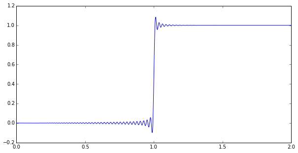
Impressed? Maybe you should be. This is a goal that’s been bugging the heck out of me for a few months, and I’ve finally reached something useful.
Let’s start with a quick overview.
1. Denial
Padé Approximants
If you’ve done any studying of linear time-invariant (LTI) systems, you know that the transfer function of a time delay T is \( H(s) = e^{-sT} \). An exponential function. Very simple, but it’s kind of an oddball. That’s because most transfer functions are written as a ratio of polynomials \( H(s) = \frac{P(s)}{Q(s)} \) — in other words a rational function — and analyzed by standard techniques to find their poles and zeros and do some sort of numerical calculation with them. So we can’t find the “poles” of \( H(s) = e^{-sT} \), because there aren’t any. Huh.
Okay, so what do we do instead?
If you’re using Simulink to model something, it’s fine to just add a time delay. Simulink has some secret recipe for handling time delays and it works just fine.
But what if you want to perform some kind of continuous-time analysis where you need a rational transfer function? Well, you could try to convert everything to a discrete-time approximation, where a time delay is very easy and becomes a shift in a state variable array. Or you can approximate a continuous-time delay with a rational function. And whenever you see the words “approximate… rational function”, the first thing that should come to mind is Padé approximation. This is a technique to compute the “closest” rational function to a given function using power series. It’s kind of the rational-function equivalent to a Taylor series — it’s based upon the function and its derivatives at a single point — and if you’ve read my article on Chebyshev approximation, you’ll know I don’t particularly like Taylor series, but it has its place, and so does Padé approximation. Padé approximation has a reputation for being a “magic” solution that somehow captures more of the essence of a smooth function than a power series, with a wider range of convergence. Let’s look at a mildly interesting example: \( f(x) = 10 \tan^{-1} (x-2) + \frac{2}{x} \) near \( x=1 \).
import numpy as np
import scipy
import matplotlib.pyplot as plt
%matplotlib inline

def f(x):
    return 10*np.arctan(x-2) + 2.0/x

x = np.arange(-3,5,0.002)
# fixup plot so it doesn't draw an extra line across a discontinuity
def asymptote_nan(y,x,x0list):
    x0list = np.atleast_1d(x0list)
    for x0 in x0list:
        y[np.argmin(abs(x-x0))] = float('nan')
    return y
y = asymptote_nan(f(x),x,x0list=[0])
fig = plt.figure(figsize=(8,6))
ax = fig.add_subplot(1,1,1)
ax.plot(x,y)
ax.set_ylim(-40,40)
ax.grid('on')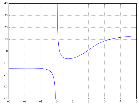
We can use scipy to figure out numerical coefficients of a Taylor series and the Padé approximations, using scipy.interpolate.approximate_taylor_polynomial and scipy.misc.pade: (warning: scipy.misc.pade expects its input coefficients to be in order of ascending degree, whereas the return values of both functions are numpy.poly1d objects that yield coefficients in order of descending degree. Hence the T10.coeffs[::-1] expression to reverse the order.)
import scipy.interpolate
import scipy.misc

x0 = 1.0
T10poly = scipy.interpolate.approximate_taylor_polynomial(f,x=x0,degree=10, scale=0.05)
P5poly,Q5poly = scipy.misc.pade(T10poly.coeffs[::-1],5)
T10 = lambda x: T10poly(x-x0)
R5_5 = lambda x: P5poly(x-x0)/Q5poly(x-x0)
fig = plt.figure(figsize=(8,6))
ax = fig.add_subplot(1,1,1)
ax.plot(x,y,label='f(x)')
ax.plot(x0,f(x0),'.k',markersize=8)
yR5 = R5_5(x)
# use real roots of Q5(x-x0) for finding asymptotes
yR5 = asymptote_nan(yR5, x, [r+x0 for r in roots(Q5poly) if np.abs(np.imag(r)) < 1e-8])
ax.plot(x,T10(x),label='T10(x)')
ax.plot(x,yR5, label='R5,5(x)')
ax.set_ylim(-40,40)
ax.legend(loc='lower right',labelspacing=0)
ax.grid('on')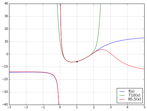
So there’s an example of Padé magic. The rational function does a better job than the polynomial. Why is that a big deal?
Well, the two functions \( T_{10}(x) \) and \( R_{5,5}(x) = P_5(x)/Q_5(x) \) each have 11 degrees of freedom: \( T_{10} \) has 11 coefficients, \( P_5 \) and \( Q_5 \) each have 6 coefficients but we lose one degree of freedom since we can scale \( P_5 \) and \( Q_5 \) by the same arbitrary constant \( K \) and leave the resulting rational function unchanged. Moreover, we derived \( T_{10} \) directly from \( f(x) \), but derived \( R_{5,5} \) from \( T_{10} \). So there’s no additional “information” in \( R_{5,5} \) beyond what’s in \( T_{10} \), just some freedom of structure, since \( T_{10} \) is required to be a polynomial whereas \( R_{5,5} \) is a rational function.
But \( R_{5,5} \) has a much wider range of applicability than \( T_{10} \): while \( T_{10} \) is a decent approximation to \( f(x) \) over a range of about \( x \in [0.2, 1.9] \), the function \( R_{5,5} \) looks very good over the range \( x \in [-3, 2.3] \). And here’s the kicker: somehow the function \( R_{5,5}(x) \) “knows” about the discontinuity at \( x=0 \) just from looking at the polynomial \( T_{10}(x) \). We lost the pole at \( x=0 \) going from \( f(x) \) to the Taylor series \( T_{10}(x) \), but somehow got it back when we used Padé approximation to go from \( T_{10}(x) \) to the rational function \( R_{5,5}(x) \). Magic!
In the words of the authors of Numerical Recipes (see page 202):
Padé has the uncanny knack of picking the function you had in mind from among all the possibilities. Except when it doesn’t!
The structure of a rational function usually lets it do a better job of approximating, but sometimes it doesn’t. Anyway, this article isn’t really about Padé approximation in general, but about the use of Padé approximation for time delays.
Time Delays and Padé Approximants
The Padé approximation \( R_{p,q}(x) = \frac{N_{p,q}(x)}{D_{p,q}(x)} \approx e^{-x} \) is well-known, and its coefficients can be determined exactly using these formulas (see Moler and Van Loan for a reputable reference for \( e^A \)):
$$ \begin{eqnarray} N_{p,q}(x) &=& \sum\limits_{j=0}^p\frac{(p+q-j)!p!}{(p+q)!j!(p-j)!}(-x)^j \cr D_{p,q}(x) &=& \sum\limits_{j=0}^q\frac{(p+q-j)!q!}{(p+q)!j!(q-j)!}x^j \cr \end{eqnarray} $$
Here the numerator \( N_{p,q}(x) \) has degree \( p \) and denominator \( D_{p,q}(x) \) has degree \( q \). The expression \( n! \) denotes n factorial, namely the product of all positive integers between 1 and \( n \), so \( 5! = 5 \times 4 \times 3 \times 2 \times 1 = 120 \). The various combinations of \( p \) and \( q \) can be used to show the various approximations in tabular form, known as a Padé table. Just for some examples,
$$ \begin{array}{ll} R_{1,1}(x) = \frac{1 - \frac{1}{2}x} {1 + \frac{1}{2}x} & R_{1,2}(x) = \frac{1 - \frac{1}{3}x} {1 + \frac{2}{3}x + \frac{1}{6}x^2} & R_{1,3}(x) = \frac{1 - \frac{1}{4}x} {1 + \frac{3}{4}x + \frac{1}{4}x^2 + \frac{1}{24}x^3} \cr R_{2,1}(x) = \frac{1 - \frac{2}{3}x + \frac{1}{6}x^2} {1 + \frac{1}{3}x} & R_{2,2}(x) = \frac{1 - \frac{1}{2}x + \frac{1}{12}x^2} {1 + \frac{1}{2}x + \frac{1}{12}x^2} & R_{2,3}(x) = \frac{1 - \frac{2}{5}x + \frac{1}{20}x^2} {1 + \frac{3}{5}x + \frac{3}{20}x^2 + \frac{1}{60}x^3} \cr R_{3,1}(x) = \frac{1 - \frac{3}{4}x + \frac{1}{4}x^2 - \frac{1}{24}x^3} {1 + \frac{1}{4}x} & R_{3,2}(x) = \frac{1 - \frac{3}{5}x + \frac{3}{20}x^2 - \frac{1}{60}x^3} {1 + \frac{2}{5}x + \frac{1}{20}x^2} & R_{3,3}(x) = \frac{1 - \frac{1}{2}x + \frac{1}{10}x^2 - \frac{1}{120}x^3} {1 + \frac{1}{2}x + \frac{1}{10}x^2 + \frac{1}{120}x^3} \cr \end{array}$$
which can be seen in the following semilogarithmic graph:
fig = plt.figure(figsize=(10,6))
ax = fig.add_subplot(1,1,1)
x = np.arange(-5,5,0.0005)
ax.semilogy(x,np.exp(-x),'--',label='e^-x')
ax.grid('on')

def pade_coeffs(p,q):
    '''
    Calculate the numerator and denominator
    polynomial coefficients of the Pade
    approximation to e^-x
    '''
    n = max(p,q)
    c = 1
    d = 1
    clist = [c]
    dlist = [d]
    for k in xrange(1,n+1):
        c *= -1.0*(p-k+1)/(p+q-k+1)/k
        if k <= p:
            clist.append(c)
        d *= 1.0*(q-k+1)/(p+q-k+1)/k
        if k <= q:
            dlist.append(d)
    return np.array(clist[::-1]),np.array(dlist[::-1])

def argbox(y,ymin,ymax,imin,imax):
    '''
    find limits (we hope)
    where y[i] is between ymin and ymax
    '''
    ii = np.argwhere(np.logical_and(y>ymin,y<ymax))
    ii = ii[ii >= imin]
    ii = ii[ii <= imax]
    return np.min(ii),np.max(ii)

nx = len(x)
xmin = min(x)
xmax = max(x)
xlim = (xmin,xmax)
ylim = (1e-4,1e4)
for p in [1,2,3]:
    for q in [1,2,3]:
        pcoeffs, qcoeffs = pade_coeffs(p,q)
        P = np.poly1d(pcoeffs)
        Q = np.poly1d(qcoeffs)
        num = P(x)
        den = Q(x)
        ax.semilogy(x,num/den,label='p=%d, q=%d' % (p,q))
        # now label the end lines
        it = argbox(num/den, ylim[0], ylim[1], 0, nx/2)[0]
        atend = it == 0
        xt = x[it] * (0.99 if atend else 1)
        yt = P(xt)/Q(xt) if atend else ylim[1]*0.95
        ax.text(xt,yt,' (%d,%d)' % (p,q), va='top',
                rotation='horizontal' if atend else -90.0)
        it = argbox(num/den, ylim[0], ylim[1], nx/2, nx)[1]
        atend = it == (nx-1)
        xt = x[it] * (0.99 if atend else 1)
        yt = P(xt)/Q(xt) if atend else ylim[0]*1.2
        ax.text(xt,yt,'(%d,%d)' % (p,q), va='bottom',
                ha='right' if atend else 'left',
                rotation='horizontal' if atend else -90.0)
ax.set_xlim(xlim)
ax.set_ylim(ylim)
ax.set_xlabel('x')
ax.set_ylabel('y = f(x)')
ax.legend(labelspacing=0)
<matplotlib.legend.Legend at 0x107935810>
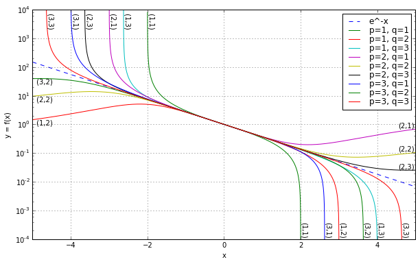
Increasing either \( p \) or \( q \) expands the region of close convergence by a little bit.
But we were talking about simulating time delays. So we don’t really care too much about \( e^{-x} \) for real values of \( x \); instead we care about Bode plots of \( e^{-s} \) for \( s=j\omega \).
w = np.arange(0,10,0.001)
s = 1j*w
fig = plt.figure(figsize=(10,6))

for k in [1,2]:
    ax = fig.add_subplot(2,1,k)
    if k == 1:
        f = lambda H: 20*np.log10(np.abs(H))
        ylabel = '$20\\,\\log_{10} |H(j\\omega)|$'
    else:
        f = lambda H: np.unwrap(np.angle(H))*180/np.pi
        ylabel = '$\\angle H(j\\omega)$'
        ax.set_yticks(np.arange(-720,0.01,45))
        ax.set_xlabel('$\omega$', fontsize=16)
        ax.plot(w,-w*180/np.pi,'--',label='e^jw')
    for q in [1,2,3]:
        for p in np.arange(1,q+1):
            pcoeffs, qcoeffs = pade_coeffs(p,q)
            P = np.poly1d(pcoeffs)
            Q = np.poly1d(qcoeffs)
            H = P(s)/Q(s)
            ax.plot(w,f(H),label='p=%d,q=%d' % (p,q))
    ax.set_ylabel(ylabel, fontsize=16)
    ax.grid('on')
    ax.legend(loc='best', labelspacing=0)
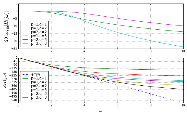
These are Bode plots, but linear rather than logarithmic in frequency, so that we can compare to \( e^{-s} \) which has a unity gain and linear phase responses. Here we are only using \( p \leq q \), otherwise the gain increases as \( \omega \rightarrow \infty \), which is not realizable. When \( p = q \), the gain is 1, independent of frequency. The higher \( p \) and \( q \) are, the more the phase response approaches the ideal \( e^{-s} \) for larger frequencies. Looks great, right?
Let’s try using the Padé coefficients in the time domain, with scipy.signal.lti to simulate the step responses:
import scipy.signal

t = np.arange(0,3,0.001)
fig = plt.figure(figsize=(10,6))
ax = fig.add_subplot(1,1,1)
ax.set_xlabel('t')
ax.plot(t,t>=1,'--k')
for q in [1,2,3]:
    for p in np.arange(1,q+1):
        pcoeffs, qcoeffs = pade_coeffs(p,q)
        P = np.poly1d(pcoeffs)
        Q = np.poly1d(qcoeffs)
        H = scipy.signal.lti(P,Q)
        _,y = H.step(T=t)
        ax.plot(t,y,label='p=%d,q=%d' % (p,q))
ax.grid('on')
ax.legend(loc='best', labelspacing=0)
<matplotlib.legend.Legend at 0x105479e10>
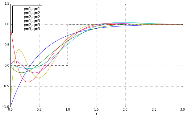
Well, that doesn’t look very satisfying. Not even close to a step. This is the problem with time ↔ frequency transforms; if something looks great in the time domain it usually looks bad in the frequency domain, and vice-versa.
Let’s just look at the \( p=q \) case since the degree of the transfer function denominator is the main determining factor in realizability; once we’ve decided, for example, that we’re going to use a 7th degree polynomial denominator, it doesn’t really matter much for realization purposes whether the numerator is just 1 or it’s a 6th or 7th degree polynomial. And for a fixed-degree denominator, the higher degree numerator does a better job of approximating \( e^{-s} \). Besides, when you see implementations of Padé approximations, like in MATLAB, they’re usually just using \( p=q \). This gives a unity gain at all frequencies (“all-pass”) without any low-pass-filtering.
Here’s the step responses for the first 10 \( p=q \) Padé approximations to a unit delay:
import scipy.signal

t = np.arange(0,3,0.001)
fig = plt.figure(figsize=(10,6))
ax = fig.add_subplot(1,1,1)
ax.set_xlabel('t')
ax.plot(t,t>=1,'--k')
for q in np.arange(1,11):
    p = q
    pcoeffs, qcoeffs = pade_coeffs(p,q)
    P = np.poly1d(pcoeffs)
    Q = np.poly1d(qcoeffs)
    H = scipy.signal.lti(P,Q)
    _,y = H.step(T=t)
    ax.plot(t,y,label='p=q=%d' % q)
ax.grid('on')
ax.legend(loc='best', labelspacing=0)
<matplotlib.legend.Legend at 0x1087c7b10>
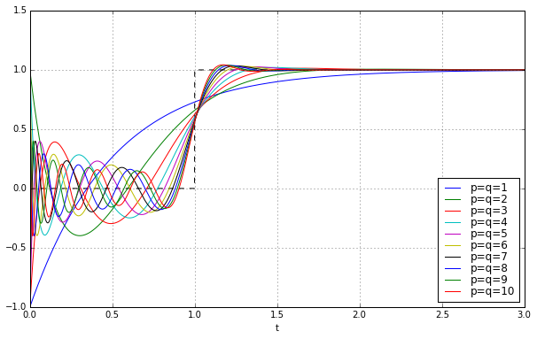
They get better as \( q \) increases, but there’s still this nasty jump near \( t=0 \), and ringing between \( t=0 \) and \( t=1 \) that’s kind of like the phenomenon of Gibbs ears in partial Fourier sums to approximate a square wave.
But still, that’s kind of cool; we can approximate a time delay with a rational transfer function.
Great! So let’s use just keep on going in degree:
import scipy.signal

t = np.arange(0,3,0.001)
fig = plt.figure(figsize=(10,6))
ax = fig.add_subplot(1,1,1)
ax.set_xlabel('t')
ax.plot(t,t>=1,'--k')
for q in [5,10,15,20,21,22]:
    p = q
    pcoeffs, qcoeffs = pade_coeffs(p,q)
    P = np.poly1d(pcoeffs)
    Q = np.poly1d(qcoeffs)
    H = scipy.signal.lti(P,Q)
    _,y = H.step(T=t)
    ax.plot(t,y,label='p=q=%d' % q)
ax.set_ylim(-0.5,2.5)
ax.grid('on')
ax.legend(loc='best', labelspacing=0)
<matplotlib.legend.Legend at 0x1055b8d50>
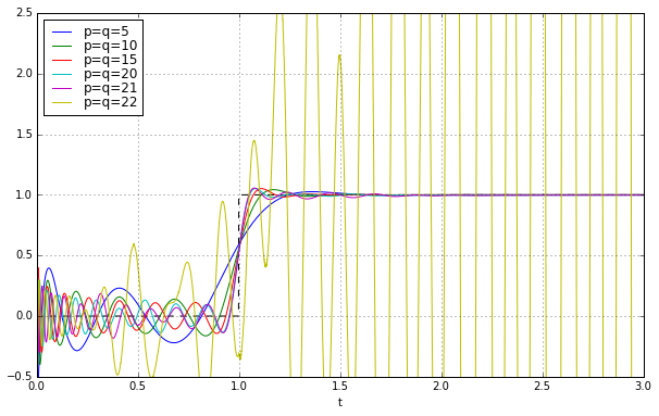
Uh oh. Things look good until about \( q=21 \), and then BAM! we get instability. The footnote in MATLAB’s Padé approximation says this:
High-order Padé approximations produce transfer functions with clustered poles. Because such pole configurations tend to be very sensitive to perturbations, Padé approximations with order
N>10should be avoided.
And maybe four or five years ago, when I was last messing around with Padé approximations for a time delay, I left it at that. Because why would you need a high-order Padé approximation anyway? It’s rare to have systems where there’s a time delay but no additional high-frequency rolloff, and when you add that, the ringing doesn’t look as bad. Here’s the step response of a unit time delay cascaded in series with a 1-pole low-pass filter. We’ll show time constants 0.1, 0.2, 0.5, and 1.0, and we’ll look at the exact answer and some Padé approximations of order 5, 10, and 15.
t = np.arange(0,4,0.001)
Tdelay = 1.0
for tau in [0.1, 0.2, 0.5, 1.0]:
    fig = plt.figure(figsize=(10,6))
    ax = fig.add_subplot(1,1,1)
    ax.set_xlabel('t')
    y_exact = (t>Tdelay)*(1-np.exp(-(t-Tdelay)/tau))
    ax.plot(t,y_exact,'--k',label='exact')
    for q in [5,10,15]:
        p = q
        pcoeffs, qcoeffs = pade_coeffs(p,q)
        P = np.poly1d(pcoeffs)
        Q = np.poly1d(qcoeffs)
        H = scipy.signal.lti(P,Q)
        _,y = H.step(T=t)
        # 1-pole LPF
        _,y2,_ = scipy.signal.lsim([[1/tau],[1, 1/tau]],y,t)
        ax.plot(t,y2,label='p=q=%d' % q)
    ax.set_ylim(-0.1,1.1)
    ax.grid('on')
    ax.legend(loc='best', labelspacing=0)
    ax.text(1.1*Tdelay,0,'tau=%.2f' % tau, fontsize=16)
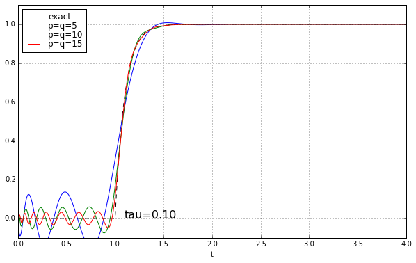
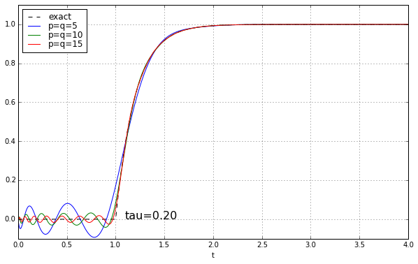
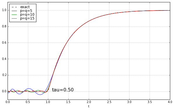
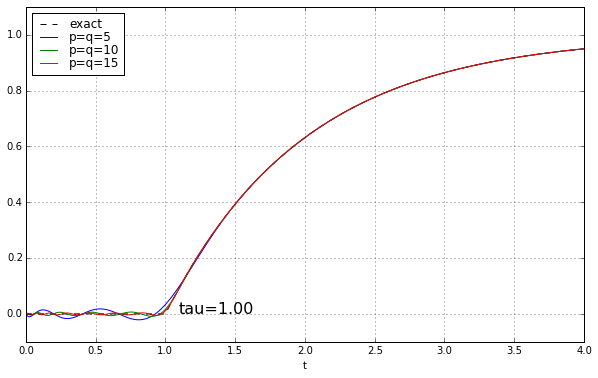
The longer the time constant, the less relevant are those ripples from the time-delay approximation.
See? There’s no problem here. No problem at all.
2. Anger
But then a few months ago I needed to get the step response (in a Simulink-free manner) for some systems that had time delays that weren’t very small, and I needed to know if the ripples were due to numerical simulation issues or they were real, so a clean response was important. Grrr.
Padé Problems: Take Two
Something’s fishy here. MathWorks says we should avoid orders more than 10, but the step responses of \( q=15 \) and \( q=20 \) look reasonable. Let’s take a look at this “clustered poles” explanation by plotting the poles and zeros:
import scipy.signal

t = np.arange(0,3,0.001)
fig = plt.figure(figsize=(10,10))
ax = fig.add_subplot(1,1,1)
for q in [5,10,15,20,25]:
    p = q
    pcoeffs, qcoeffs = pade_coeffs(p,q)
    P = np.poly1d(pcoeffs)
    Q = np.poly1d(qcoeffs)
    H = scipy.signal.lti(P,Q)

    #poles = np.roots(qcoeffs)
    #zeros = np.roots(pcoeffs)
    poles = H.poles
    zeros = H.zeros
    for z,m in [(poles,'x'),(zeros,'o')]:
        ax.plot(np.real(z),np.imag(z),'.k',marker=m,mfc='none')
plt.axis('equal')
ax.set_xlim(-50,50)
ax.set_ylim(-50,50);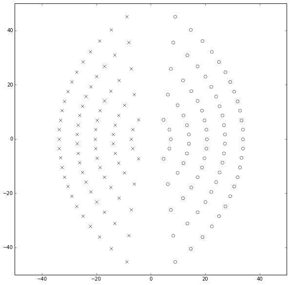
Huh — that doesn’t look bad. The poles and zeros are symmetric for \( p=q \) and line up along arcs that get further away from the origin as the value of \( q \) increases. I don’t see any “clustering” here, and we’re showing values up to \( p=q=25 \).
So why do we get instability in simulation?
It really depends on how simulations are implemented. For scipy.signal.lti, the key is that time-domain simulations (lsim, step, impulse, etc.) depend on state-space representation of an LTI system. This means we rely on converting from transfer function form (arrays of numerator and denominator polynomial coefficients) to state-space via tf2ss. How does tf2ss work?
Pigs in State-Space
Here’s a sample system: let’s look at \( H(s) = \frac{P(s)}{Q(s)} = \frac{1}{(s+1)(0.5s+1)(0.2s+1)(0.1s+1)} = \frac{100}{s^4 + 18s^3 + 97s^2 + 180s + 100} \):
ABCD = scipy.signal.tf2ss([100],[1,18,97,180,100])
for k,suffix in enumerate('ABCD'):
    print '%s=\n%s' % (suffix, ABCD[k])
A= [[ -18. -97. -180. -100.] [ 1. 0. 0. 0.] [ 0. 1. 0. 0.] [ 0. 0. 1. 0.]] B= [[ 1.] [ 0.] [ 0.] [ 0.]] C= [[ 0. 0. 0. 100.]] D= [ 0.]
What’s all this A B C D stuff anyway?
State-space is a representation for LTI systems using matrices, that has a couple of advantages over the rational transfer function approach we tend to learn in introductory control systems courses. One is that it can be used to model multi-input multi-output (MIMO) systems. Another is that we can transform a multi-order scalar differential equation (e.g. \( \frac{d^4y}{dt^4} + 18\frac{d^3y}{dt^3} + 97\frac{d^2y}{dt^2} + 180\frac{dy}{dt} + 100y = 100u \)) into a first-order matrix differential equation. It can simulate aspects of systems (non-controllable / non-observable systems) that aren’t easily modeled with transfer functions. It’s also more amenable to computerized analysis, and it has some numerical advantages over the transfer function approach that we’ll look at in a bit.
An LTI state-space system looks like this:
$$ \begin{eqnarray} \frac{d}{dt}\mathbf x &=& A\mathbf x + B\mathbf u \cr \mathbf y &=& C\mathbf x + D\mathbf u \end{eqnarray} $$
where \( \mathbf u \) is a vector of input signals, \( \mathbf x \) is a vector of internal state signals (which is why it’s called state-space) and \( \mathbf y \) is a vector of output signals. You can still use state-space in the SISO case, in which case \( u \) and \( y \) are scalar values but \( \mathbf x \) remains a vector of length equal to the order of the system. In our example case, we have
$$ \begin{eqnarray} A &=& \begin{bmatrix} -18 & -97 & -180 & -100 \cr 1 & 0 & 0 & 0 \cr 0 & 1 & 0 & 0 \cr 0 & 0 & 1 & 0 \cr \end{bmatrix} \cr B &=& \begin{bmatrix} 1 & 0 & 0 & 0 \cr \end{bmatrix}^T \cr C &=& \begin{bmatrix} 0 & 0 & 0 & 100 \end{bmatrix} \cr D &=& 0 \end{eqnarray} $$
The \( A \) matrix here has a particular structure. It’s a variant of what’s called a companion matrix of the monic denominator polynomial \( Q(x) \) of the transfer function (monic just means that the term of highest degree has a coefficient of 1); what’s special about it is
- the first row is -1 times the coefficients of \( Q(x) \) aside from the leading coefficient
- the subdiagonal elements are 1, and the remaining elements are 0, forming a shift matrix in the lower rows
- the characteristic polynomial of the companion matrix is equal to \( Q(x) \), meaning its eigenvalues are equal to the roots of \( Q(x) \)
Furthermore — and this applies to any square matrix \( A \) — if all the eigenvalues, which are equal to the roots of \( Q(x) \), are distinct, then \( A \) is similar to any other matrix \( M \) with the same eigenvalues, meaning that there is some transformation matrix \( T \) such that \( M = T^{-1}AT \), and \( A \) is diagonalizable, meaning it can be factored as \( A = V\Lambda V^{-1} \) where \( V \) is a matrix of eigenvectors and \( \Lambda \) is the diagonal matrix of corresponding eigenvalues.
Matrix matrix eigenblahblahblah — if you’re not familiar or comfortable with linear algebra, this stuff will just make your eyes glaze over. (Especially when you ask how to obtain the transfer function, which ends up being \( H(s) = C(sI-A)^{-1}B + D \); computing the inverse term gets ugly very quickly, and this equation always makes me think of some obscure Hungarian mathematician for some reason.) Don’t worry; I’ll walk you through the implications.
In our particular example, the state equation can be written out as
$$ \frac{d\mathbf x}{dt} = \frac{d}{dt} \begin{bmatrix} \frac{d^3x}{dt^3} \cr \frac{d^2x}{dt^2} \cr \frac{dx}{dt} \cr x \end{bmatrix} = \begin{bmatrix} -18 & -97 & -180 & -100 \cr 1 & 0 & 0 & 0 \cr 0 & 1 & 0 & 0 \cr 0 & 0 & 1 & 0 \cr \end{bmatrix} \begin{bmatrix} \frac{d^3x}{dt^3} \cr \frac{d^2x}{dt^2} \cr \frac{dx}{dt} \cr x \end{bmatrix} + \begin{bmatrix}1 \cr 0 \cr 0 \cr 0\end{bmatrix} u = A\mathbf x + B u $$
so in this representation of the transfer function, the elements of the state vector are just a scalar state variable \( x \) with transfer function \( \frac{1}{Q(s)} = \frac{x(s)}{u(s)} \), and the first \( n-1 \) derivatives of \( x \). The \( n-1 \) bottom rows fall out from the relation between successive elements of the state vector: each element is the derivative of the next element. And the top row is self-evident from the differential equation relating \( x \) and \( u \).
This is called the controllable canonical form, which tf2ss uses, and its main virtue is that it is easy to construct the \( A \), \( B \), \( C \), and \( D \) matrices directly from the transfer function. It has some lousy properties, though.
Betrayal: The Perils of Polynomial Coefficients and the Companion Matrix
For symbolic analysis of LTI systems, use of the companion matrix is fine. But things can get ugly if we try to use them in numerical analysis.
The problems start because of finite computational precision and something called conditioning, which measures the relative error gain from “input” to “output”, where “input” and “output” here are interpreted loosely, depending on the context. Usually when someone talks about ill-conditioning, it’s in the context of solving the linear matrix equation \( Ax=b \) for \( x \), in which case the condition number is \( \kappa(A) = \|A\| \cdot \|A^{-1}\| \) — this involves matrix norms, which you can read about at your leisure. When solving \( Ax=b \), it means that if I have some relative error \( \epsilon_b \) in \( b \), the relative error \( \epsilon_x \) in the solution \( x \) can be bounded by \( \epsilon_x \leq \kappa(A) \epsilon_b \), so the condition number \( \kappa(A) \) represents a error magnification ratio.
For example, if you have the ill-conditioned equation
$$Ax = \begin{bmatrix} 2&1 \cr 4&1.998 \end{bmatrix}\begin{bmatrix}x_1 \cr x_2\end{bmatrix} = b$$
where \( \kappa(A) \approx 6248 \), the solution for \( b = [1,2]^T \) is \( x_1 = 0.5, x_2 = 0 \). If we have \( b = [0.99,2]^T \), a small change, the solution shifts drastically to \( x_1 = -4.495, x_2 = 10 \). The problem input \( b \) only changed by a relative error of \( 0.01/\sqrt{5} \approx 0.004472 \), whereas the problem output \( x \) changed by a relative error of \( \sqrt{4.995^2 + 10^2}/0.5 \approx 22.3562 \) — a magnification factor of 4999.
Ill-conditioning in numerical analysis is kind of like the biomagnification of mercury in fish, only worse. If you eat a lot of tuna, the mercury content in your body can accumulate to a higher concentration than it was in the tuna, which in turn had higher concentrations than in the fish eaten by the tuna.

There’s not a practical way of removing the mercury once it’s in the fish. But you can control how much of it you eat, and the human body does get rid of it (albeit very slowly). Whereas once you have introduced numerical errors into mathematical calculations, there’s rarely any way to get rid of them. Let me say this again: Numerical errors are even worse than toxic poison! The best way to avoid their problems is to keep them out of your system in the first place; once they’ve made their way into calculations it’s too late. And unfortunately, ill-conditioned numerical problems are error magnets that turn the very small but unavoidable errors of floating-point calculations into large errors.
Anyway, the sensitivity of solving linear systems is only one way to define condition numbers. Another is to look at sensitivity of the roots of a polynomial given its coefficients.
For example, let’s take \( Q(s) = s^4 + 18s^3 + 97s^2 + 180s + 100 \) and find the sensitivity of its roots to the non-leading coefficients. There are four roots and four non-leading coefficients, so we can find a 4 × 4 matrix of sensitivities. If we increase the last coefficient by \( 1+\delta \) with \( \delta = 0.0001 \) (from 100 to 100.01), the roots change from \( [-10, -5, -2, -1] \) to approximately \( [-9.99997222, -5.00016666, -1.99958324, -1.00027788] \), which is a relative change of approximately \( \delta \times [-0.02777811, 0.33331204, -2.08380389, 2.77882873] \). This is the first column of a sensitivity matrix, and we can repeat the same thing for the other three columns:
Q = np.poly1d([1,18,97,180,100])

def find_root_sensitivities(Q, delta=1e-10, extras=False):
    """
    Returns a relative sensitivity matrix S from coefficients to roots.
    If extras is True, returns S, kappa, v, with:

      kappa = the norm of the sensitivity matrix

      v = a unit vector of maximum sensitivity which produces sensitivity gain kappa
    """
    Q = np.poly1d(Q)
    n = Q.order
    roots = np.roots(Q)
    S = np.zeros((n,n), dtype=roots.dtype)   # allow for complex numbers
    for k in xrange(n):
        # find approx numerical derivative
        # from symmetric differences
        Qplus = Q*1.0
        Qminus = Q*1.0
        Qplus[k] *= (1+delta/2.0)
        Qminus[k] *= (1-delta/2.0)
        rplus = np.roots(Qplus)
        rminus = np.roots(Qminus)
        if np.any(np.iscomplex(rplus)) or np.any(np.iscomplex(rminus)):
            S = S.astype(np.complex128)
        S[:,k] = (np.roots(Qplus) - np.roots(Qminus)) / roots / delta
    if not extras:
        return S
    # extras: find a direction of maximum sensitivity
    u,s,v = np.linalg.svd(S, compute_uv=True)
    # largest singular direction in reverse order
    # to match polynomial coefficients n-1:0
    return S,s[0],v[0,::-1]

S,kappa,v = find_root_sensitivities(Q, extras=True)
S,kappa,v
(array([[-0.02777334, 0.50001248, -2.69444733, 4.99999508],
[ 0.33334402, -3.00002156, 8.08333667, -7.49996509],
[-2.08332684, 7.50000284, -8.08332734, 2.99997693],
[ 2.7777769 , -5.00000152, 2.69445133, -0.49999782]]),
17.015155693892876,
array([-0.48543574, 0.70522631, -0.49695306, 0.14158266]))# double-check that this direction vector v works: # if we perturb the coefficients towards v and away from v, # we should be able to see that the magnitude of change # in the coefficient vector is amplified by kappa to yield # a larger magnitude of change in the root vector Qplus = Q*1.0 Qminus = Q*1.0 r = np.roots(Q) delta = 1e-10 Qplus.coeffs[1:] *= 1+v*delta/2.0 Qminus.coeffs[1:] *= 1-v*delta/2.0 rplus = np.roots(Qplus) rminus = np.roots(Qminus) dr = (rplus - rminus)/r/delta print dr np.linalg.norm(dr,2)
[ -4.57977833 10.8794147 -11.17900439 5.02097586]
17.015180620416512
We can adjust each non-leading coefficient \( c_k \) by some relative factor \( 1 + v_k\delta \), where \( \sum |v_k|^2 = 1 \) and \( \delta \) is a magnitude of adjustment. The resulting measure of relative change of the roots \( R = \sqrt{\sum |\delta r_k|^2} \) where \( \delta r_k \) is the relative change in each root. If we choose the \( v_k \) appropriately (and it turns out that we can obtain \( v_k \) by calculating the singular value decomposition of the sensitivity matrix \( S = U\Sigma V \), and then take \( v_k \) as the first row of \( V \)), then we can get the maximum value of \( R = \kappa \delta \): the root-sum-square of relative changes in the roots, is equal to the root-sum-square of relative changes in the coefficients, magnified by this factor \( \kappa \) which is the Euclidean norm of the sensitivity matrix, and can be considiered as a condition number because it tells the relative gain of input error to output error.
For our example, \( Q(s) = s^4 + 18s^3 + 97s^2 + 180s + 100 \), \( \kappa \approx 17.015 \). Numerical errors in the coefficients produces numerical errors in the roots that, depending on the direction, can be as much as just over 17.015 times as large.
All monomials (1st-degree polynomials) have \( \kappa = 1 \), but as the degree of a polynomial increases, the condition number of its roots generally increases to a very large number. For example, the 10th-degree polynomial \( P_{10}(x) = \prod\limits_{k=1}^{10} (x-\frac{1}{k}) \), the condition number \( \kappa \) is over a million. In fact, it’s difficult to estimate this condition number accurately.
P10 = 1.0
for k in xrange(1,11):
    P10 = P10*np.poly1d([1, -1.0/k])
P10
poly1d([ 1.00000000e+00, -2.92896825e+00, 3.51454365e+00,
-2.31743276e+00, 9.41614308e-01, -2.48582176e-01,
4.34780093e-02, -5.00165344e-03, 3.63756614e-04,
-1.51565256e-05, 2.75573192e-07])S,kappa,v = find_root_sensitivities(P10, extras=True) kappa
1586991.6991524738
This matters because small changes in polynomial coefficients can produce large changes in the roots. In fact, polynomial coefficients expressed as floating-point numbers are a really lousy way to analyze and evaluate polynomials unless the polynomial degree is small. Let that sink in for a moment: Large degree polynomials specified by floating-point coefficients are poorly conditioned for numerical analysis. (And by “large”, we’re talking above the 5-10 degree range, depending on the application.)
In terms of simulation, this is important: the roots of the transfer function’s denominator polynomial determine the dynamics of the system, and high sensitivity of these roots to errors in coefficients (which is how we specify the \( A \) matrix in tf2ss) make simulating high-degree transfer functions very error-prone.
We can look at the root sensitivity condition number for the \( (p,q) \) Padé approximation of a unit time delay, as a function of the polynomial degree:
for n in [5,10,15,20,25]:
    pcoeffs, qcoeffs = pade_coeffs(n,n)
    Q = np.poly1d(qcoeffs)
    S,kappa,v = find_root_sensitivities(Q, extras=True)
    print 'n=%d, kappa=%g' % (n,kappa)
n=5, kappa=71.3885 n=10, kappa=28069.6 n=15, kappa=1.43265e+07 n=20, kappa=8.28673e+09 n=25, kappa=1.52504e+11
OUCH! No wonder the transfer function approach fails for large degree polynomials. This really stinks. In fact, if we continue to try to compute the poles and zeros of the Padé approximations from their coefficients, the results start to become inaccurate above about degree 25. Plotting those results looks like a marching band about to go berserk:
import scipy.signal

t = np.arange(0,3,0.001)
fig = plt.figure(figsize=(10,10))
ax = fig.add_subplot(1,1,1)
for q in [22,24,26,28,30,32]:
    p = q
    pcoeffs, qcoeffs = pade_coeffs(p,q)
    P = np.poly1d(pcoeffs)
    Q = np.poly1d(qcoeffs)
    H = scipy.signal.lti(P,Q)

    #poles = np.roots(qcoeffs)
    #zeros = np.roots(pcoeffs)
    poles = H.poles
    zeros = H.zeros
    for z,m in [(poles,'x'),(zeros,'o')]:
        ax.plot(np.real(z),np.imag(z),'.k',marker=m,mfc='none')
plt.axis('equal')
ax.set_xlim(-60,60)
ax.set_ylim(-60,60);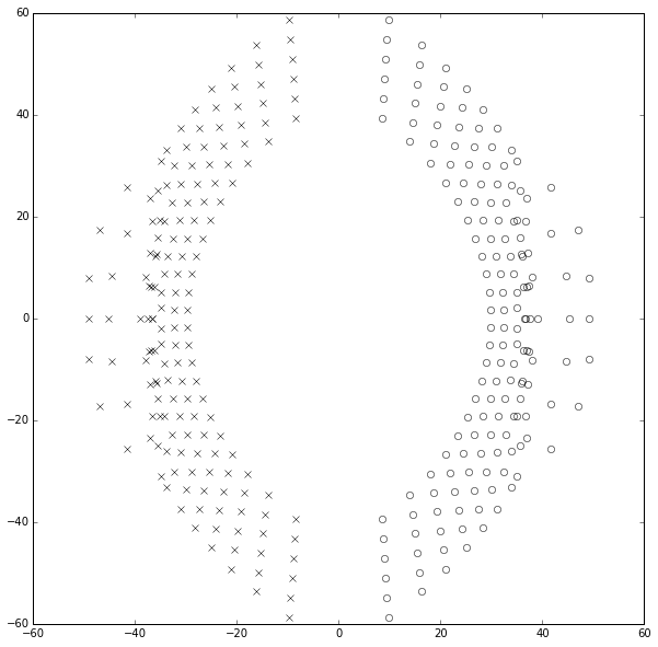
The scipy simulation functions (lsim, step, impulse, etc.) for scipy 0.15.x and earlier are even worse in this regard than finding roots of polynomials, because they try to diagonalize the \( A \) matrix as \( A = V\Lambda V^{-1} \), which has its own problems at large degree. For example, if we diagonalize the companion matrix of the 10th degree polynomial \( P_{10}(x) = \prod\limits_{k=1}^{10} (x-\frac{1}{k}) \), we get an eigenvector matrix \( V \) that has a condition number of more than \( 10^{11} \), whereas the eigenvalue sensitivity we computed earlier was only about 1.59 million.
A10=np.polynomial.polynomial.polycompanion(P10.coeffs[::-1])
Lambda,V = np.linalg.eig(A10)
print '%g' % np.linalg.cond(V)
1.36681e+11
Drat. Drat drat drat.
3. Bargaining
Throwing Polynomial Coefficients out the Window
Well, if one major cause of problems is the expression of transfer functions as a pair of polynomials by listing their coefficients, then maybe there’s another way to make them work.
There are other ways to describe polynomials. Two of them which don’t suffer from the ill-conditioned problems of polynomial coefficients are
- factoring polynomials — write a polynomial as a product \( P(x) = A\prod\limits_{k=0}^{n}(x-r_k) \) rather than a sum \( P(x) = \sum\limits_{k=0}^{n} a_kx^k \)
- sum of Chebyshev polynomials — write \( P(x) = \sum\limits_{k=0}^{n} c_kT_k(u) \) with \( u = \frac{2x-a-b}{b-a} \) to scale \( x \in [a,b] \) to \( u \in [-1,1] \)
Chebyshev polynomials \( T_k(u) \) work well because they are bounded between \( \pm 1 \) and don’t run into the numerical problems we get when we evaluate large powers of \( x \) that partially cancel each other out. Evaluating them from the recurrence relation \( T_n(u) = 2uT_{n-1}(u) - T_{n-2}(u) \) is numerically stable. But they only work well in a bounded range \( x \in [a,b] \). If we have an unbounded range then they won’t help.
So factoring is another approach. But then we have to find the roots of the polynomials. And the formulas we have for the Padé approximation to \( e^{-s} \) give us the coefficients; we already know finding the roots from coefficients is a badly-conditioned problem. If we have to start from coefficients, the poison is already there, and we’re dead in the water.
Zeros of the Hypergeometric Function \( {}_1F_1 \)
Both the numerator and the denominator of the Padé approximation to \( e^{-s} \) have the same form, which can be written in terms of the hypergeometric function \( {}_1F_1(a;b;z) \):
$$ \begin{eqnarray} N_{p,q}(x) &=& \sum\limits_{j=0}^p\frac{(p+q-j)!p!}{(p+q)!j!(p-j)!}(-x)^j &=& {} _ 1F_1 (-p;-p-q;-x)\cr D_{p,q}(x) &=& \sum\limits_{j=0}^q\frac{(p+q-j)!q!}{(p+q)!j!(q-j)!}x^j &=& {} _ 1F_1 (-q;-p-q;x)\cr \end{eqnarray} $$
Now we just need a way to find the zeros of these functions so we can dispense with having to deal with their coefficients.
There are tons of obscure mathematical papers on the zeros of special functions; Saff and Varga’s 1975 paper On the Zeros and Poles of Padé Approximants to \( e^x \) prove theorems about the locations of the poles and zeros in the complex plane, but say nothing about how to numerically compute them.
After a bunch of floundering around, I found two very interesting papers that are relevant to finding these poles and zeros:
- Rafael G. Campos and Marisol L. Calderón, Approximate Closed-Form Formulas for the Zeros of the Bessel Polynomials
- F. Alberto Grünbaum, Variations on a theme of Heine and Stieltjes: an electrostatic interpretation of the zeros of certain polynomials
Campos and Calderón’s paper on the Bessel polynomials explore a different special function, but they have the same general problem and they make a rather off-hand remark about finding zeros using a property of the Bessel polynomials:
$$\sum\limits_{k\neq j}\frac{1}{z_j - z_k} + \frac{az_j + 2}{2z_j^2} = 0$$
This set of nonlinear equations can be solved by standard methods. We have used a Newton method to solve them up to \( n=500 \) and \( a=100 \).
This intrigued me — they found roots of a 500th degree polynomial using some equations and Newton’s method — but it was unclear how to repeat the approach or adapt it to the Padé approximants.
Grünbaum’s article states that for any polynomials with simple (nonrepeated) roots,
If $$P(x)=(x-x_1)(x-x_2)\ldots (x-x_n)$$ then at any root \( x_k \) of \( P \) we have $$P’‘(x_k) = 2P’(x_k)\sum\limits_{j \neq k}\frac{1}{x_k-x_j}$$
This means that at any root \( x_k \), then
$$\frac{P’‘(x_k)}{2P’(x_k)} = \sum\limits_{j \neq k}\frac{1}{x_k-x_j}$$
For our Padé polynomials, the Wikipedia page on \( {}_1F_1 \) has \( w={}_1F_1(a;b;z) \) satisfying the differential equation
$$z \frac{d^2w}{dz^2} + (b-z)\frac{dw}{dz} - aw = 0$$
and at the roots where \( w=0 \),
$$z \frac{d^2w}{dz^2} + (b-z)\frac{dw}{dz} = 0$$
so that
$$ \frac{\frac{d^2w}{dz^2}}{2\frac{dw}{dz}} = \frac{z-b}{2z} $$
Therefore, at all zeros \( x_k \) of the denominator polynomial \( D_{p,q}(x) = w={}_1F_1(a=-q;b=-p-q;x) \), we have
$$0 = -\frac{1}{2} + \frac{-p-q}{2x_k} + \sum\limits_{j\neq k}\frac{1}{x_k-x_j}$$.
There are \( q \) of these equations and they can each be treated as one component of a vector equation \( \mathbf F(\mathbf v) = \mathbf 0 \) where \( \mathbf v \) is the set of the \( x_k \) roots. The Newton-Raphson method applied to vector equations is that if we have some estimate \( \mathbf v[m] \), we can calculate the next estimate \( \mathbf v[m+1] \) as follows:
- calculate \( \mathbf y = \mathbf F(\mathbf v[m]) \)
- calculate the Jacobian matrix \( \mathbf J = \frac{\partial \mathbf F}{\partial \mathbf v} \) evaluated at \( \mathbf v[m] \)
- solve for \( \Delta \mathbf v \) where \( \mathbf J \Delta \mathbf v = \mathbf y \)
- calculate \( \mathbf v[m+1] = \mathbf v[m] - \Delta \mathbf v \)
We also need an initial guess; some empirical messing around trying to approximate the zeros for \( D_{p,q}(x) \) in the q=10-20 range led me to the initial guess
$$ \mathbf v[0] = -p - \frac{q}{3} + \frac{2q}{3}\mathbf u^2 + \frac{2j(p+q)}{3}\mathbf u $$
where \( \mathbf u \) is the vector with the \( k \)th component \( u_k = \frac{2k - (q-1)}{q} \) for \( k = 0 \ldots q-1 \) — this leads to the \( u_k \) nearly spanning the range \( (-1,1) \) — and \( \mathbf u^2 \) is the element-by-element square of the vector \( \mathbf u \).
This approach actually surprisingly well. What I don’t understand is why it converges to the right answer, rather than getting stuck at some other solution or running into some numerical problems due to ill-conditioning; Newton’s methods can be very iffy and don’t always converge well. But in this case it can easily be used to get the poles and zeros for \( p \) and \( q \) in the range of several hundred. (The numerator \( N_{p,q}(x) \) has the same exact method and its vector of zeros \( v \) are equal to -1 times the zeros of the denominator polynomial with \( p \) and \( q \) swapped.)
And here’s an example of it in action with \( p=200, q=200 \):
import sspade

def plotpolezero(z,p,ax=None):
    if ax is None:
        fig = plt.figure(figsize=(8,8))
        ax = fig.add_subplot(1,1,1, aspect='equal')
    ax.plot(np.real(z),np.imag(z),'ok',markersize=3,mfc='none')
    ax.plot(np.real(p),np.imag(p),'xk',markersize=3)
    return ax

ax=None
for q in [25,50,75,100,125,150,175,200]:
    pe = sspade.PadeExponential(q,q)
    zeros, poles, k = pe.zpk
    ax=plotpolezero(zeros,poles,ax)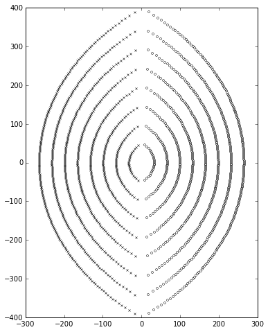
Things get more interesting if we look at \( p<q \); if \( p \) is small enough, some of the poles can drift into the right half-plane, indicating an unstable system:
ax=None
for p in [15,20,25,30,35,40]:
    pe = sspade.PadeExponential(p,40)
    zeros, poles, k = pe.zpk
    ax=plotpolezero(zeros,poles,ax)
ax.grid('on')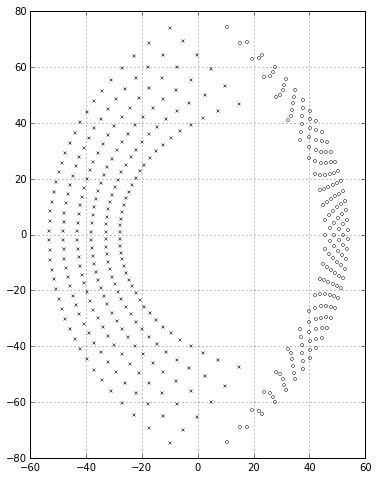
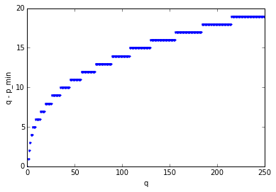
The minimum value \( p_{min}(q) \) that produces all poles in the left half-plane is less than but close to \( q \); if we graph \( q - p_{min}(q) \) we get values that gradually increase:
pminlist = []
qlist = np.arange(250)
p = 0
for q in qlist:
    pprev = p
    while p < q:
        pe = sspade.PadeExponential(p,q)
        zeros,poles,k = pe.zpk
        if np.all(np.real(poles) < 0):
            break
        else:
            p += 1
    if (q-1 - pprev) < (q-p):
        print p,q
    pminlist.append(p)
plt.plot(qlist, qlist-pminlist,'.')
plt.xlabel('q')
plt.ylabel('q - p_min')
0 0 0 1 0 2 0 3 0 4 1 6 3 9 7 14 11 19 17 26 25 35 34 45 45 57 59 72 75 89 93 108 114 130 139 156 166 184 196 215
<matplotlib.text.Text at 0x104c57950>
Let’s shift our attention back to actually trying to use the Padé approximation. Now that we can find the poles and zeros using Newton’s method, we can avoid the ill-conditioned poison of the polynomial coefficient expression, and start using it in the frequency domain even for large values of \( p \) and \( q \), since it’s just a matter of evaluating the transfer function at the frequencies of our choice. The phase angle of the transfer function \( \frac{N_{p,q}(s)}{D_{p,q}(s)} \) roughly matches a pure unit time delay \( e^{-s} \) up to a frequency of approximately \( \omega = p+q \); here’s a graph showing the \( p=q \) case up to \( p=q=120 \):
w = np.arange(0,300,0.01)
s = 1j*w
plt.plot(w,-w, ':', label='e^-s')
for q in [20,40,60,80,100,120]:
    pe = sspade.PadeExponential(q,q)
    plt.plot(w,np.unwrap(np.angle(pe(s))), label='(p=q=%d)' % q)
plt.xlabel('$\\omega$', fontsize=16)
plt.ylabel('$\\angle H(j\\omega)$, radians', fontsize=16)
plt.legend(loc='lower left', labelspacing=0);
The tough part is going to be dealing with our system in the time domain. We have the technology, though, now that we can get the poles and zeros without having to go through the polynomial coefficients.
4. Depression
Okay, so now the question is how we setup a linear system for time-domain simulation. If you look at the documentation for scipy.signal.lti, you’ll see that
The lti class can be instantiated with either 2, 3 or 4 arguments. The following gives the number of elements in the tuple and the interpretation: - 2: (numerator, denominator) - 3: (zeros, poles, gain) - 4: (A, B, C, D)
Each argument can be an array or sequence.
So we’ll just use the 3-argument constructor so we can utilize the zero, poles, gain triple directly:
t = np.arange(0,3,0.001)
fig = plt.figure(figsize=(10,6))
ax = fig.add_subplot(1,1,1)
ax.set_xlabel('t')
ax.plot(t,t>=1,'--k')
for q in [18,20,22]:
    pe = sspade.PadeExponential(q,q)
    zeros, poles, k = pe.zpk
    H = scipy.signal.lti(zeros, poles, k)
    _,y = H.step(T=t)
    ax.plot(t,y,label='p=q=%d' % q)
ax.grid('on')
ax.legend(loc='best', labelspacing=0)
ax.set_ylim(-0.5,1.2);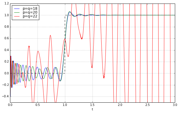
Huh? We’re in trouble again at \( p=q=22 \). What’s going on?
The key here is how scipy.signal.lti handles simulations. This behavior changed between version 0.15 and version 0.16, but in both cases simulation always utilizes the (A,B,C,D) state-space form, and if the system is specified in one of the other two methods (numerator/denominator coefficient vectors, or ZPK = zero-pole-gain), it is converted to state-space first.
In version 0.15 the calculation of the state-space matrices in the scipy.signal.lti class goes through the _update method which, in the case of ZPK, calls zpk2ss:
def _update(self, N):
    if N == 2:
        self._zeros, self._poles, self._gain = tf2zpk(self.num, self.den)
        self._A, self._B, self._C, self._D = tf2ss(self.num, self.den)
    if N == 3:
        self._num, self._den = zpk2tf(self.zeros, self.poles, self.gain)
        self._A, self._B, self._C, self._D = zpk2ss(self.zeros,
                                                    self.poles, self.gain)
    if N == 4:
        self._num, self._den = ss2tf(self.A, self.B, self.C, self.D)
        self._zeros, self._poles, self._gain = ss2zpk(self.A, self.B,
                                                      self.C, self.D)
This is promising, but then if we look at zpk2ss, we see this:
def zpk2ss(z, p, k):
    """Zero-pole-gain representation to state-space representation
    Parameters
    ----------
    z, p : sequence
        Zeros and poles.
    k : float
        System gain.
    Returns
    -------
    A, B, C, D : ndarray
        State space representation of the system, in controller canonical
        form.
    """
    return tf2ss(*zpk2tf(z, p, k))
We call zpk2tf which goes from zero-pole-gain form to transfer function coefficients, and then call tf2ss. Horrors! That’s right — we went to great lengths to avoid polynomial coefficients because of their ill-conditioning, and instead work directly with the poles and zeros, but zpk2ss throws all that care away and goes right back to the error-prone polynomial coefficient approach.
Version 0.16 has been refactored to separate classes for each form of construction, and the ZeroPolesGain class has a to_ss method that’s used in simulation:
def to_ss(self):
    """
    Convert system representation to `StateSpace`.
    Returns
    -------
    sys : instance of `StateSpace`
        State space model of the current system
    """
    return StateSpace(*zpk2ss(self.zeros, self.poles, self.gain))
And in version 0.16 it’s the same old sloppy zpk2ss function that goes through transfer function coefficients:
def zpk2ss(z, p, k):
    """Zero-pole-gain representation to state-space representation
    Parameters
    ----------
    z, p : sequence
        Zeros and poles.
    k : float
        System gain.
    Returns
    -------
    A, B, C, D : ndarray
        State space representation of the system, in controller canonical
        form.
    """
    return tf2ss(*zpk2tf(z, p, k))
It’s the same in scipy 0.17. So we lose! Dammit. Controller canonical form really sucks for numerical purposes.
The Right Way to Implement zpk2ss
We need a better way to implement zpk2ss, and since scipy won’t do it for us, we’ll have to do it ourselves. A little research on matrices easily shows that the way to keep the condition number of the \( A \) matrix to a minimum is to make it a pure diagonal matrix. Let’s go back to the 4th-order system we talked about earlier:
$$H(s) = \frac{P(s)}{Q(s)} = \frac{1}{(s+1)(0.5s+1)(0.2s+1)(0.1s+1)} = \frac{100}{s^4 + 18s^3 + 97s^2 + 180s + 100}$$
which has a controller canonical form of
$$ \begin{eqnarray} A &=& \begin{bmatrix} -18 & -97 & -180 & -100 \cr 1 & 0 & 0 & 0 \cr 0 & 1 & 0 & 0 \cr 0 & 0 & 1 & 0 \cr \end{bmatrix} \cr B &=& \begin{bmatrix} 1 & 0 & 0 & 0 \cr \end{bmatrix}^T \cr C &=& \begin{bmatrix} 0 & 0 & 0 & 100 \end{bmatrix} \cr D &=& 0 \end{eqnarray} $$
where the \( A \) matrix has a condition number of just over 521:
A,B,C,D = scipy.signal.tf2ss([100],[1,18,97,180,100])
np.linalg.cond(A)
521.33808185890325
We could diagonalize \( A = V\Lambda V^{-1} \) numerically:
Lambda,V = np.linalg.eig(A)
print "Lambda = ", Lambda
print "V ="
print V
print "V*diag(Lambda)*V.inv ="
print np.dot(np.dot(V,np.diag(Lambda)),np.linalg.inv(V))
Lambda =  [-10.  -5.  -2.  -1.]
V =
[[  9.94987442e-01  -9.79797151e-01   8.67721831e-01  -5.00000000e-01]
 [ -9.94987442e-02   1.95959430e-01  -4.33860916e-01   5.00000000e-01]
 [  9.94987442e-03  -3.91918861e-02   2.16930458e-01  -5.00000000e-01]
 [ -9.94987442e-04   7.83837721e-03  -1.08465229e-01   5.00000000e-01]]
V*diag(Lambda)*V.inv =
[[ -1.80000000e+01  -9.70000000e+01  -1.80000000e+02  -1.00000000e+02]
 [  1.00000000e+00   4.27435864e-15   1.19904087e-14  -3.55271368e-15]
 [  1.04083409e-17   1.00000000e+00   1.02140518e-14   3.55271368e-15]
 [  2.42861287e-17   5.55111512e-17   1.00000000e+00  -8.88178420e-16]]
But then we’ve already picked up the poison of ill-conditioning, by working with controller canonical form. It works okay for small matrices, but we shouldn’t have much hope above \( n=10 \) or so.
Instead we have to diagonalize things analytically, and that means working through the modal form, which uses a diagonal \( A \) matrix with elements equal to the transfer function poles:
$$ A = \begin{bmatrix} -10 & 0 & 0 & 0 \cr 0 & -5 & 0 & 0 \cr 0 & 0 & -2 & 0 \cr 0 & 0 & 0 & -1 \cr \end{bmatrix} $$
Now the only hard part is coming up with \( B \) and \( C \) matrices to make things work properly. There isn’t a unique choice here; we just need to make sure that the net transfer function \( H(s) = C(sI-A)^{-1}B + D \) is what we need, and for a diagonal matrix, the \( (sI-A)^{-1} \) term is also a diagonal matrix with terms \( \frac{1}{s+p} \) along the diagonal:
$$ (sI-A)^{-1} = \begin{bmatrix} \frac{1}{s+10} & 0 & 0 & 0 \cr 0 & \frac{1}{s+5} & 0 & 0 \cr 0 & 0 & \frac{1}{s+2} & 0 \cr 0 & 0 & 0 & \frac{1}{s+1} \cr \end{bmatrix} $$
The reason to use modal form is that with modes as state variables, there is no cross-coupling between modes, and in the time domain each state variable represents an independent first-order system. Very easy to analyze! As far as figuring out the \( B \) and \( C \) matrices goes, since \( (sI-A)^{-1} \) is diagonal with terms \( \frac{1}{s+p_k} \), any choice of \( B \) and \( C \) is fine that satisfies \( H(s) = \sum\limits_k \frac{b_kc_k}{s+p_k} \). We need to compute the residue coefficients \( r_k \) such that \( H(s) = \sum\limits_k \frac{r_k}{s+p_k} \) and divide up factors \( r_k \) between \( B \) and \( C \) as desired: for example, taking \( B \) as all ones and \( c_k = r_k \), or \( C \) as all ones and \( b_k = r_k \), or make them identical as \( b_k = c_k = \sqrt{r_k} \).
In our specific fourth-order case, we can use the Heaviside method to determine the residues as
$$\begin{eqnarray} a _ 0 &=& \left.\frac{100}{(s+1)(s+2)(s+5)}\right| _ {s=-10} = -\frac{5}{18} \cr a _ 1 &=& \left.\frac{100}{(s+1)(s+2)(s+10)}\right| _ {s=-5} = \frac{5}{3} \cr a _ 2 &=& \left.\frac{100}{(s+1)(s+5)(s+10)}\right| _ {s=-2} = -\frac{25}{6} \cr a _ 3 &=& \left.\frac{100}{(s+2)(s+5)(s+10)}\right| _ {s=-1} = \frac{25}{9} \end{eqnarray}$$
and therefore if we take \( B = \begin{bmatrix}1 & 1 & 1 & 1\end{bmatrix}^T \), then \( C = \begin{bmatrix}-\frac{5}{18} & \frac{5}{3} & -\frac{25}{6} & \frac{25}{9}\end{bmatrix} \), which we can verify:
H2 = scipy.signal.lti(diag([-10,-5,-2,-1]),
                 [[1]]*4,
                 [-5.0/18, 5.0/3, -25.0/6, 25.0/9],
                 0
                 )
print 'num=',H2.num
print 'den=',H2.den
print 'cond(A)=',np.linalg.cond(H2.A)
num= [[ 0.00000000e+00 -1.06581410e-14 -8.52651283e-14 -1.13686838e-13
1.00000000e+02]]
den= [ 1. 18. 97. 180. 100.]
cond(A)= 10.0
The modal form expresses any state-space system as the parallel sum of separate first-order systems; the condition number of the \( A \) matrix is just the ratio of the largest and smallest eigenvalue magnitudes. Actual physical systems rarely have only real poles, but rather at least one pair of complex conjugate eigenvalues, so we have to be cautious with this approach, because it means the \( A \), \( B \), and \( C \) matrices will have complex coefficients; an alternative is to group any complex poles in conjugate pairs and use a block-diagonal \( A \) matrix with block elements that are either 1x1 for real poles, or 2x2 of the form \( \begin{bmatrix}-\sigma&\omega\cr-\omega&-\sigma\end{bmatrix} \), which has eigenvalues \( -\sigma\pm j\omega \). This yields real-valued matrices and can be used with all of the scipy functions; some of them don’t work well with complex-valued state-space matrixes.
Okay, so let’s do it; in the sspade.PadeExponential class I’ve included properties lti_ssmodal (pure diagonal state-space matrix) and lti_ssrealmodal (block diagonal state-space matrix):
t = np.arange(0,3,0.001)
fig = plt.figure(figsize=(10,6))
ax = fig.add_subplot(1,1,1)
ax.set_xlabel('t')
ax.plot(t,t>=1,'--k')
for q in [18,20,22]:
    pe = sspade.PadeExponential(q,q)
    zeros, poles, k = pe.zpk
    H = pe.lti_ssrealmodal
    _,y = H.step(T=t)
    ax.plot(t,y,label='p=q=%d' % q)
ax.grid('on')
ax.legend(loc='best', labelspacing=0)
ax.set_ylim(-0.5,1.2);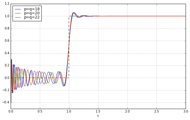
Wheeeeeee!!!!!!!!! It works! Let’s march onward to higher degree:
t = np.arange(0,3,0.001)
fig = plt.figure(figsize=(10,6))
ax = fig.add_subplot(1,1,1)
ax.set_xlabel('t')
ax.plot(t,t>=1,'--k')
for q in [20,22,24,26,28]:
    pe = sspade.PadeExponential(q,q)
    zeros, poles, k = pe.zpk
    H = pe.lti_ssrealmodal
    _,y = H.step(T=t)
    ax.plot(t,y,label='p=q=%d' % q)
ax.grid('on')
ax.legend(loc='best', labelspacing=0)
ax.set_ylim(-0.5,1.2);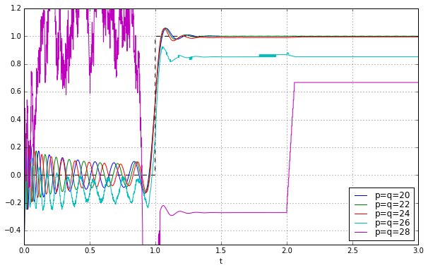
Oh, it doesn’t work. Argh.... after a bunch of looking around, I noticed the lsim2 and step2 functions, which use ODE solvers to simulate; the lsim and step functions try to be smart and use closed-form solutions to linear systems (relying on matrix exponentials), and this works better for some systems but causes numerical problems in others, and high-order systems is one of those times.
So let’s use scipy.signal.step2 instead:
t = np.arange(0,3,0.001)
fig = plt.figure(figsize=(10,6))
ax = fig.add_subplot(1,1,1)
ax.set_xlabel('t')
ax.plot(t,t>=1,'--k')
for q in [20,22,24,26,28]:
    pe = sspade.PadeExponential(q,q)
    zeros, poles, k = pe.zpk
    H = pe.lti_ssrealmodal
    H.D = np.array(1)    # TODO: FIX FIX FIX
    _,y = scipy.signal.step2(H,T=t)
    ax.plot(t,y,label='p=q=%d' % q)
ax.grid('on')
ax.legend(loc='best', labelspacing=0)
ax.set_ylim(-0.5,1.2);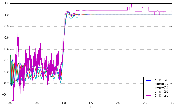
We managed to push things out further by another 4 degrees, to \( p=q=24 \); it’s borderline stable at \( p=q=26 \), and then fails at higher values.
Damn, damn, damn.
5. Acceptance…?
After I managed to figure out how to compute poles and zeros of high-order Padé time delay approximations using Newton’s method, I spent a very long day trying to get the ZPK implementation working, first stymied by the implementation of scipy‘s zpk2ss, and then in a failed attempt at a modal form implementation.
It took me a long time to figure out why the modal form doesn’t work, even though the condition number of the \( A \) matrix is much lower:
pe = sspade.PadeExponential(12,12)
zeros,poles,k = pe.zpk
H1 = scipy.signal.lti(zeros, poles, k)
H2 = pe.lti_ssrealmodal
print "controller canonical form K(A)=%g" % np.linalg.cond(H1.A)
print "modal form K(A)=%g" % np.linalg.cond(H2.A)
controller canonical form K(A)=1.63807e+15
modal form K(A)=1.28474
Wow. The modal form has a condition number of 1.28 for \( p=q=12 \), whereas the controller canonical form has a condition number of over \( 10^{15} \). The modal form shouldn’t be causing us numerical problems at all.... but the problem is that the ill-conditioning has been “swept aside” into the \( B \) and \( C \) matrices:
print "B="
print H2.B
print "C="
print H2.C
B=
[[   18.05591692]
 [  132.91771897]
 [  851.69993802]
 [  304.37549706]
 [ 2894.68914148]
 [ 2500.50514786]
 [ 3177.55610818]
 [-1303.54031239]
 [ 1898.61079121]
 [  126.23776885]
 [ -223.46066064]
 [   37.6807615 ]]
C=
[[   18.05591692   132.91771897   851.69993802   304.37549706
   2894.68914148  2500.50514786 -3177.55610818  1303.54031239
  -1898.61079121  -126.23776885   223.46066064   -37.6807615 ]]
My implementation uses \( b_k = c_k = \sqrt{r_k} \) to reduce magnitudes, but there’s still a delicate cancellation between modes. Each of the modes is oscillating at its own characteristic frequency, most of them with a relatively large amplitude, and they are supposed to sum up to small values. This doesn’t work too well once the system order gets fairly large:
for q in [16,18,20,22,24]:
    pe = sspade.PadeExponential(q,q)
    zeros,poles,k = pe.zpk
    H2 = pe.lti_ssrealmodal
    print "C_%d=" % q
    print H2.C
C_16=
[[ 1.55868479e+01 5.19857547e+02 2.04887023e+03 2.57337115e+03
1.82882935e+04 7.10695442e+03 4.31275008e+04 3.60662991e+04
-4.50120393e+04 2.09511572e+04 -3.21075818e+04 -6.80395204e+02
7.59499100e+03 -1.63614662e+03 2.48124131e+02 6.35855671e+01]]
C_18=
[[ 6.59640301e+01 1.13979997e+02 3.42432615e+03 1.23189110e+04
1.02201903e+04 7.85142459e+04 3.08958948e+04 1.65125772e+05
1.36577005e+05 -1.69418842e+05 8.21961937e+04 -1.28145915e+05
-3.50145127e+02 3.68157292e+04 -8.01311715e+03 2.46639032e+03
-8.02882151e+02 -4.43317147e+01]]
C_20=
[[ 7.71477361e+01 1.09480088e+03 2.20976889e+03 1.89068039e+04
6.52104021e+04 3.93204917e+04 3.27775187e+05 1.29770199e+05
6.30151994e+05 5.16584425e+05 -6.37675797e+05 3.19757062e+05
-5.05485067e+05 6.73972798e+03 1.68214908e+05 -3.63903841e+04
1.72063240e+04 -6.14389658e+03 -1.86962826e+02 5.54803332e+01]]
C_22=
[[ 2.92848728e+01 6.92739882e+02 9.76114462e+03 1.95615111e+04
9.45543017e+04 3.19193112e+05 1.48199173e+05 1.34170005e+06
5.32633296e+05 2.39897177e+06 1.95222307e+06 -2.40016773e+06
1.23634882e+06 -1.97709719e+06 5.41285003e+04 7.38679949e+05
-1.57696485e+05 1.01020692e+05 -3.78633338e+04 5.91146021e+02
1.31571948e+03 -1.08300118e+02]]
C_24=
[[ 1.30410652e+02 1.35369198e+03 3.24570356e+03 6.70668054e+04
1.32333628e+05 4.44087115e+05 1.48231772e+06 5.50774714e+05
5.41332494e+06 2.15076021e+06 9.11611817e+06 7.37282635e+06
-9.03411488e+06 4.75871679e+06 -7.68407951e+06 3.05267070e+05
3.15357164e+06 -6.62292235e+05 5.35078004e+05 -2.06529518e+05
1.42833365e+04 1.38783403e+04 -1.40768237e+03 -1.29015506e+01]]
The modal form has good numerical stability in the \( A \) matrix, but sacrifices numerical stability in the system as a whole, so unfortunately it’s not a good choice either.
Cascade
The right choice is a cascade (series) implementation. If we can break down the system into 1st- and 2nd-order systems with appropriate eigenvalues that can be cascaded into a high-order system, then we don’t require additive cancellation between modes.
The algebra of cascaded state-space implementations is as follows:
If we have two state-space systems \( S_1 = (A_1, B_1, C_1, D_1) \) and \( S_2 = (A_2, B_2, C_2, D_2) \) such that the inputs of \( S_2 \) are the outputs of \( S_1 \), then the combined system \( S_{12} = (A_{12}, B_{12}, C_{12}, D_{12}) \) can be computed as
$$ \begin{eqnarray} A_{12} &=& \begin{bmatrix}A_1 & 0 \cr B_2C_1 & A_2\end{bmatrix} \cr B_{12} &=& \begin{bmatrix}B_1 \cr B_2D_1 \end{bmatrix} \cr C_{12} &=& \begin{bmatrix}D_2C_1 & C_2\end{bmatrix} \cr D_{12} &=& D_2D_1 \cr \end{eqnarray} $$
This cascade combination can be continued to more than two systems; for example, the three-system cascade looks like this:
$$ \begin{eqnarray} A_{123} &=& \begin{bmatrix}A_1 & 0 & 0 \cr B_2C_1 & A_2 & 0 \cr B_3D_2C_1 & B_3C_2 & A_3\end{bmatrix} \cr B_{123} &=& \begin{bmatrix}B_1 \cr B_2D_1 \cr B_3D_2D_1\end{bmatrix} \cr C_{123} &=& \begin{bmatrix}D_3D_2C_1 & D_3C_2 & C_3\end{bmatrix} \cr D_{123} &=& D_3D_2D_1 \cr \end{eqnarray} $$
And the four-system cascade looks like this:
$$ \begin{eqnarray} A_{1234} &=& \begin{bmatrix}A_1 & 0 & 0 & 0\cr B_2C_1 & A_2 & 0 & 0 \cr B_3D_2C_1 & B_3C_2 & A_3 & 0 \cr B_4D_3D_2C_1 & B_4D_3C_2 & B_4C_3 & A_4 \end{bmatrix} \cr B_{1234} &=& \begin{bmatrix}B_1 \cr B_2D_1 \cr B_3D_2D_1 \cr B_4D_3D_2D_1\end{bmatrix} \cr C_{1234} &=& \begin{bmatrix}D_4D_3D_2C_1 & D_4D_3C_2 & D_4C_3 & C_4\end{bmatrix} \cr D_{1234} &=& D_4D_3D_2D_1 \cr \end{eqnarray} $$
In general, the resulting cascaded state-space system has an \( A \) matrix which is block lower triangular; if the \( D \) terms are zero then it’s block lower bidiagonal. The condition number of this matrix isn’t as low as with the modal form (though still much lower than controller canonical form!), but overall it’s much more stable:
pe = sspade.PadeExponential(12,12)
zeros,poles,k = pe.zpk
H3 = pe.lti_sscascade
print "cascade form K(A) = ", np.linalg.cond(H3.A)
print H3.C
cascade form K(A) =  7056.31427616
[[ -66.02737609 -628.04637117  -63.9781648  -196.10488621  -59.72456992
  -102.02762662  -52.888034    -56.65414163  -42.63766873  -28.21917019
   -26.74418646   -8.83087886]]
So finally we can try our time-delay step response with high-order systems using a cascaded implementation:
t = np.arange(0,2,0.001)
fig = plt.figure(figsize=(10,6))
ax = fig.add_subplot(1,1,1)
ax.set_xlabel('t')
ax.plot(t,t>=1,'--k')
for q in [20,40,60,80,100]:
    pe = sspade.PadeExponential(q,q)
    zeros, poles, k = pe.zpk
    H = pe.lti_sscascade
    _,y = scipy.signal.step2(H,T=t)
    ax.plot(t,y,label='p=q=%d' % q)
ax.grid('on')
ax.legend(loc='best', labelspacing=0)
ax.set_ylim(-0.1,1.1);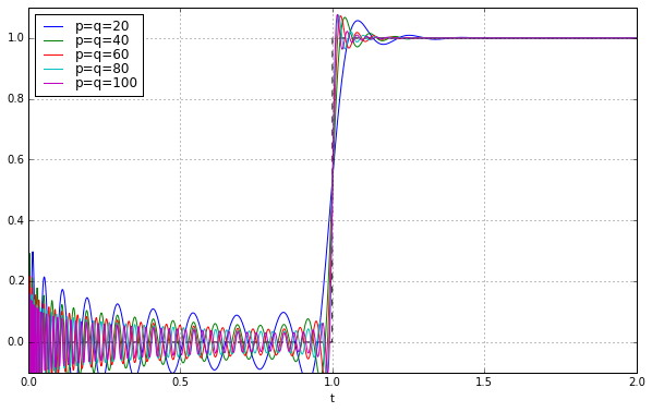
SUCCESS! We did it!
We can reduce the ringing during the delay time (with a minor increase in ringing after the delay time) if we use a slightly lower order polynomial in the numerator of the transfer function:
t = np.arange(0,2,0.001)
fig = plt.figure(figsize=(10,6))
ax = fig.add_subplot(1,1,1)
ax.set_xlabel('t')
ax.plot(t,t>=1,'--k')
for q in [20,40,60,80,100]:
    p = q-4
    pe = sspade.PadeExponential(p,q)
    zeros, poles, k = pe.zpk
    H = pe.lti_sscascade
    _,y = scipy.signal.step2(H,T=t)
    ax.plot(t,y,label='p=%d, q=%d' % (p,q))
ax.grid('on')
ax.legend(loc='best', labelspacing=0)
ax.set_ylim(-0.1,1.1);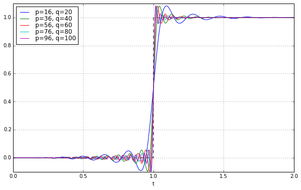
And that’s pretty much all there is to say here....
Taking it further
Hmmm. The overshoot is kind of annoying, though, isn’t it? What if, instead of taking all 100 poles and putting them into a time delay, we put some of them into a very slight low-pass filter to attenuate the ripples?
We have to be careful here, because most sharp-cutoff low-pass filters introduce more overshoot rather than less overshoot. The best one to use is probably a Bessel filter, for two reasons:
- it has very little overshoot
- it has a very flat group delay; in the passband the frequency-dependence of time delay is very low
There’s another reason too; the transfer function of a Bessel filter happens to be the same as the \( p=q \) Padé approximation to a time delay, but with a numerator of 1, and the cutoff frequency scaled by a factor of \( \frac{1}{2} \). (There’s those pesky hypergeometric functions again!) So we already have all the machinery to construct a state-space system for Bessel filters.
B5 = sspade.Bessel(5, 1.0)
print "5th order unit Bessel filter denominator polynomial"
Bp5 = np.poly(B5.poles)
assert np.all(np.imag(Bp5)<1e-12)
print np.real(Bp5)

B = sspade.Bessel(10, 1.0)
H = B.lti_sscascade
_,y = scipy.signal.step2(H,T=t)
plt.plot(t,y);
5th order unit Bessel filter denominator polynomial
[   1.   15.  105.  420.  945.  945.]
A unit Bessel filter has a low-frequency group delay of 1.0, so what we can do is allocate some of the time delay to a Bessel filter and some of the time delay to a Padé delay:
a = 0.05  # 5% of the delay goes to Bessel, the rest to Pade
n = 100   # order of the whole system
m = 10    # order of the Bessel filter
peb = sspade.Bessel(m,1.0/a)
Hb = peb.lti_sscascade
pe=sspade.PadeExponential(n-m,n-m,1/(1-a))
Hp=pe.lti_sscascade
H1 = sspade.cascade(Hb,Hp)
# System #1: cascaded Bessel + Pade
t = np.arange(0,2,0.001)

# System #2: Pade only
pe2=sspade.PadeExponential(n-m,n)
H2=pe2.lti_sscascade
# System #3: Bessel only
H3=sspade.Bessel(n).lti_sscascade

fig=plt.figure(figsize=(10,10))
ax=[fig.add_subplot(2,1,k+1) for k in xrange(2)]

for label, H in [
                 ('Pade %d,%d' % (pe2.p,pe2.q), H2),
                 ('Bessel %d $\\rightarrow$ Pade %d,%d' % (m,pe.p,pe.q), H1),
                 ('Bessel %d' % n, H3)
                ]:
    _,y = scipy.signal.step2(H,T=t)
    for axk in ax:
        axk.plot(t,y,label=label)

for k in xrange(2):
    if k > 0:
        axk.set_xlim(0.9,1.1)
    ax[k].legend(loc='best')
    ax[k].set_ylim(-0.1,1.1)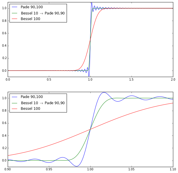
The pure Bessel filter of order 100 is very smooth but not very steep. The pure Padé filter of order 100 (with numerator degree 90) is very steep but has quite a bit of ripple. The hybrid cascade isn’t quite as steep as the Padé filter but it greatly attenuates the ripple.
The thing about the Padé filter is that it optimizes the frequency response, and comes closest to any other filter of the same numerator/denominator at meeting the frequency response of a pure time delay. But time domain and frequency domain characteristics conflict to some degree: a low-pass filter with a perfectly sharp cutoff in the frequency domain implies ripple in the time domain, and vice versa. If we were optimizing, we might want to find the order-100 IIR filter that is the best least-squared approximation to the step response of a time-shifted version of a Gaussian filter:
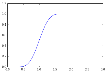
$$h(t) = \frac{1}{\sqrt{2\pi}\tau}e^{-\frac{t^2}{2\tau^2}} \leftrightarrow H(s) = \frac{1}{\sqrt{2\pi}}e^{s^2\tau^2}$$
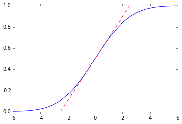
This is a noncausal filter, which has a step response \( \newcommand{\erf}{\mathop{\rm erf\,}\nolimits} y(t) = \frac{1}{2}\left(1 + \erf{\frac{t}{\sqrt{2}\tau}}\right) \) where \( \erf{x} \) is the error function; it ramps up smoothly from 0 to 1 with maximum slope \( \frac{1}{\sqrt{2\pi}\tau} \):
import scipy.special

t = np.arange(-6,6,0.001)
tau = 2.0
plt.plot(t,0.5 + 0.5*scipy.special.erf(t/np.sqrt(2)/tau))
slope = 1.0/np.sqrt(2*np.pi)/tau
plt.plot([-0.5/slope, 0.5/slope],[0,1],'--r')
plt.ylim(-0.02,1.02);
For certain particular combinations of delay/order/steepness, we can come pretty close to a Gaussian filter. The Bessel filter of order \( N \) and cutoff frequency \( f_0 \) is supposedly the best approximation to the Gaussian with time constant \( \tau = T_0/\sqrt{2N} \) and an added time delay \( T_0 = 1/f_0 \):
n=15
f0=2.5

T0=1.0/f0
tau=T0/np.sqrt(2*n)

t = np.arange(0,2,0.001)*T0
B = sspade.Bessel(n,f0)
Hb = B.lti_sscascade
_,y = scipy.signal.step2(Hb,T=t)
plt.figure(figsize=(8,6))
plt.plot(t,0.5 + 0.5*scipy.special.erf((t-T0)/np.sqrt(2)/tau))
plt.plot(t,y)
plt.ylim(-0.05,1.05)
plt.legend(['Gaussian filter tau=%.3f' % tau, 'Bessel (n=%d, f0=%.3f)' % (n,f0)],
           loc='upper left');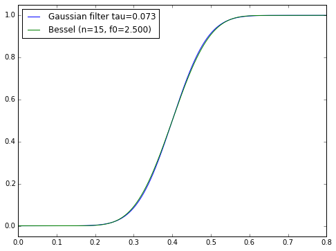
The thing is, I’m not sure if there’s a straightforward procedure for finding the best nth-order IIR filter approximation to a Gaussian filter with arbitrary time delay — where “best” here means least-squared error in the time domain. It’s one of those things that Gauss or Fourier or Legendre probably wrote a paper about some general topic, at the age of 23, of which my problem is just one special case, and they stuck it in a drawer because at the time there weren’t any applications.
So I’m just going to leave it at that.
Wrapup
- The Padé approximation to \( e^{-sT} \) (PAEST) is a rational function with specified degree \( p \) in the numerator and \( q \) in the denominator, that comes very close to matching a time delay in the frequency domain, and can be used as a rational transfer function for simulating a delay of time T.
- Padé approximation in general is similar to a Taylor series approach, but it uses rational functions instead of polynomials, and can produce a better approximation for certain functions that aren’t well-suited to polynomial approximation.
- Polynomial coefficients for this approximation are integers (for T=1 at least) and can be computed in terms of factorials or combinations using recurrence formulas.
scipy.signal.ltican be used with numerator and denominator polynomials to simulate a Padé time delay.- The low-order approximations don’t look very good (especially with \( p=q \); if \( p \) is slightly less than \( q \) they’re not too bad)
- Padé time delays don’t necessarily have to be very accurate, if they are combined with other systems that have similar or slower dynamics.
- Using
scipy.signal.ltiwith polynomial coefficients of PAEST breaks down just above order 20. - The reason this approach breaks down is because numerical conditioning of polynomial coefficients becomes TOXIC as the degree increases. (And, no, TOXIC isn’t some clever acronym, I’m just emphasizing it loudly.)
- State-space formulations of a linear system are not unique, and have several forms. The default state-space form used by
scipy.signal.ltiis the controller canonical form, which expresses a state-space system directly from the TOXIC polynomial coefficients of the transfer function numerator and denominator. - Analysis of the poles and zeros of PAEST is an end-run around ill-conditioned polynomial coefficients, and can be accomplished using Newton-Raphson iteration to obtain poles and zeros directly, with high-accuracy, based on residue sums using the second-order differential equation form for the hypergeometric function \( {}_1F_1 \).
- PAEST with \( p<q \) is unstable if \( p \) is too small, because of the presence of right-half-plane poles.
scipy.signal.ltihas a constructor that can use ZPK form (zeros, poles, DC gain) but it fails miserably becausescipy.signal.zpk2ssconverts ZPK form to TOXIC polynomial coefficients as an intermediate form before converting to state-space- We can convert poles and zeros of PAEST to state-space, but we have to take care in doing so.
- The best-conditioned state-space \( A \) matrix uses a diagonalized (“modal”) form, but this fails on most high-order systems as well, because the ill-conditioning is pushed out to the \( B \) and \( C \) matrices, and convergence relies on delicate cancellation of sums of first-order systems.
- The cascaded series form appears to be the best overall method of formulating a high-order state-space system from poles and zeros, by first grouping them into order-1 (for real poles and zeros) or order-2 (for complex conjugate poles and zeros) systems and then forming overall state-space matrices using combination formulas.
- PAEST of order 100+ works well using the cascade form with
scipy.signal.step2andscipy.signal.lsim2to simulate time-domain response. - The ripple of PAEST can be reduced greatly for a given order system, by sacrificing some bandwidth and combining with a Bessel filter.
References and other stuff
The sspade module
I’ve included the sspade Python module on my bitbucket account; it is free to use under the Apache license, and has a number of features I’ve used in this article, including these:
cascade(sys1,sys2)— computes the state-space system that is the series cascade of systemssys1andsys2zpk2ss_cascade(z,p,k)— converts ZPK = a list of zeros, poles, and DC gain, to a state-space LTI system using the cascade approach outlined in this articlezpk2ss_modal(z,p,k)— converts ZPK to a state-space LTI system using a diagonal A matrixzpk2ss_realmodal(z,p,pk)— converts ZPK to a state-space LTI system using a real block diagonal A matrix composed of at most 2x2 blocksPadeExponential(p,q,f0)— utility class for creating Padé approximations of numerator order \( p \) and denominator order \( q \) for a time delayBessel(n,f0)— utility class for creating Bessel filters
Technical references
Numerical Analysis
The classic numerical analysis books I have on my bookshelf are:
- Numerical Recipes in C, Press, Teukolsky, Vetterling, and Flannery — the math explanations are invaluable and fairly easy to understand. The C code is awful, a straight port of Fortran from the days when alphanumeric characters were a scarce resource and so variable names had to be cryptic in order to fit in memory.
- The Art of Computer Programming, Vol. 2, Donald A. Knuth. This doesn’t get into linear algebra, but the foundations of scalar floating-point arithmetic are covered here. If you can understand a section of TAOCP fully without your brain hurting, you must be a mathematician.
- Matrix Computations, Gene H. Golub and Charles Van Loan. (Also known as “Golub and Van Loan”) I have the 3rd edition. This book is dense, and if you don’t understand the basics of linear algebra you will get lost quickly, but it includes error analysis bounds and order of operation counts on many matrix algorithms.
It’s also worth reading the paper What Every Computer Scientist Should Know About Floating-Point Arithmetic by David Goldberg, which is a little bit more accessible (and more in-depth) than Knuth’s treatment, in my opinion.
These books may be useful as well to the advanced reader, and are on my to-get list — I can’t vouch for them yet, but their authors are well-reknowned.
- Accuracy and Stability of Numerical Algorithms, Nicholas J. Higham
- Applied Numerical Linear Algebra, James W. Demmel
- Numerical Linear Algebra, Lloyd N. Trefethen, and David Bau III
Linear Systems and State-Space
Sorry, I don’t have anything I can recommend here; what I’ve read is either mediocre or falls deeply into theoretical matrix hell without really coming up for air. (The Dahlehs at MIT fall into this latter category.)
Linear Systems Theory by João P. Hespanha may be of use. Chapter 1 is freely available online, and I found it useful for the various state-space interconnections. But it looks like a typical textbook overreliance on MATLAB. Oh, and I can’t stand the heading typography; textbooks shouldn’t look like ships’ logs from Star Trek.
Padé Approximants
- The Control Handbook, edited by William S. Levine; p. 80.
- Nineteen Dubious Ways to Compute the Exponential of a Matrix, Cleve Moler and Charles Van Loan. I really like reading almost any publication by Cleve Moler.
- On the Zeros and Poles of Padé Approximants to \( e^x \), E.B. Saff and R.S. Varga.
- Approximate Closed-Form Formulas for the Zeros of the Bessel Polynomials, Rafael G. Campos and Marisol L. Calderón.
- Variations on a theme of Heine and Stieltjes: an electrostatic interpretation of the zeros of certain polynomials, F. Alberto Grünbaum.
Other stuff
Dedicated to A.R., who was frequently upset.
© 2016 Jason M. Sachs, all rights reserved.


- Comments
- Write a Comment Select to add a comment
Small typo: in the extract from the Grunbaum article, where I assume you want the second derivative, you've got
where I think you want
This happens twice.
(This is what it looks like when I inspect the HTML source in my browser, after mathjax has done its work.)
you've got
’‘
where I think you want
’’

Which Hungarian mathematician are you referring to?
Not sure. :-) The CsI sequence of letters makes me think I guess of Mihaly Csikszentmihaly.
To post reply to a comment, click on the 'reply' button attached to each comment. To post a new comment (not a reply to a comment) check out the 'Write a Comment' tab at the top of the comments.
Please login (on the right) if you already have an account on this platform.
Otherwise, please use this form to register (free) an join one of the largest online community for Electrical/Embedded/DSP/FPGA/ML engineers:

