


Linear Feedback Shift Registers for the Uninitiated, Part XVIII: Primitive Polynomial Generation
Last time we figured out how to reverse-engineer parameters of an unknown CRC computation by providing sample inputs and analyzing the corresponding outputs. One of the things we discovered was that the polynomial \( x^{16} + x^{12} + x^5 + 1 \) used in the 16-bit X.25 CRC is not primitive — which just means that all the nonzero elements in the corresponding quotient ring can’t be generated by powers of \( x \), and therefore the corresponding 16-bit LFSR with taps in bits 0, 5, and 12 will not have a maximal period of \( 2^{16} - 1 \).
Some applications do require the use of primitive polynomials, and today we’re going to find them. In this article I present a hodgepodge of different methods for primitive polynomial generation. Really, we only need one — so if it seems to you like I’m trying to beat a dead horse, you’re right. Or to use another grotesque metaphor, there is more than one way to skin a cat. (No animals were harmed in the making of this article.) We’re going to start simple and then work our way up from naive to smart. Unlike the last few articles in this series, primitive polynomial generation is a mostly academic exercise, and you probably won’t find any practical use for it, but what the heck, I like this topic, and I’ve got a really cool algorithm to share — the Falling Coyote Algorithm — that I haven’t seen published anywhere else.
Tables!
Sometimes it doesn’t matter which primitive polynomials are used — you just need any primitive polynomial of a specified degree. In this case, you can just look one up in a table. There are a number of good sources.
-
Zierler and Brillhart’s On Primitive Trinomials (Mod 2) (1968) lists lots of irreducible trinomials, many of which are primitive.
- These are specified by two terms: \( n \) and \( k \). For example, the \( n=28 \) row contains \( k=1, 3, 9, 13 \), where all but \( k=1 \) are italicized, indicating that \( x^{28} + x + 1 \) is irreducible (not factorable) but not primitive, whereas \( x^{28} + x^3 + 1 \), \( x^{28} + x^9 + 1 \), and \( x^{28} + x^{13} + 1 \) are primitive.
- Tables like this typically exclude complementary polynomials: take any irreducible or primitive polynomial and reverse the coefficients, and you’ll get another irreducible or primitive polynomial, so for example \( x^{28} + x^{27} + 1 \) is irreducible, and \( x^{28} + x^{25} + 1 \), \( x^{28} + x^{19} + 1 \), and \( x^{28} + x^{15} + 1 \) are primitive.
- There are no irreducible or primitive trinomials of degrees that are multiples of 8. This is a result of Swan’s Theorem, which could be named the Curse-of-the-Octet Theorem, since you can’t use trinomials for any LFSRs which make full use of 8-bit-bytes for state storage.
- Richard Brent has also gotten into the hunt for very large primitive trinomials over \( GF(2) \). This may not mean anything to you, but he’s one of the gurus of numerical analysis. If you’re using a root-finding or maximum-finding algorithm, chances are it’s based on his research.
-
Watson’s Primitive Polynomials (Mod 2) (1962) — this lists one primitive polynomial per degree, up to degree \( n=100 \), and also \( n=107 \) and \( n=127 \) thrown in for good measure.
-
Živković‘s A Table of Primitive Binary Polynomials (1994) — this lists trinomials, pentanomials, and septanomials.
-
Arash Partow’s website — this lists all primitive polynomials up to degree 8, and many primitive polynomials for higher degrees.
-
Philip Koopman’s website — lots and lots of primitive polynomials up to degree 64 here. Just be careful you interpret the listings correctly. For example, the list of degree-5 polynomials contains
12 14 17 1B 1D 1E, and this is a different notation than I’ve been using, as it leaves out the unity term, so12hex =10010binary stands for the binary sequence100101= \( x^5 + x^2 + 1 \).
Sometimes, though, a table isn’t good enough, or you want to double-check information from the table, or something like that.
Standing on the Shoulders of Giants (Who Make Mistakes Once in a While)
A couple of years after I first heard about LFSRs, sometime around 2004 or 2005, this primitive polynomial business was bugging me. Initially I couldn’t find any source of information with a clear statement of what a primitive polynomial was, or how to find them. Then I ran across a paper that had recently been published by two Stanford professors, Saxena & McCluskey, called Primitive Polynomial Generation Algorithms Implementation and Performance Analysis. I thought it was the best thing in the world, because not only could I understand most of it, but it gave fairly easy-to-follow instructions how to go about finding primitive polynomials, and all you needed to do it efficiently was some simple matrix math. Here’s the paper’s abstract:
Performance analysis of two algorithms, MatrixPower and FactorPower, that generate all \( \varphi(2^r-1)/r \) degree-\( r \) primitive polynomials (\( \varphi \) is the Euler’s totient function) is presented. MatrixPower generates each new degree-\( r \) primitive polynomial in \( O(r^4) \sim O(r^4 \ln r) \) time. FactorPower generates each new degree-r primitive polynomial in \( O(r^4) \sim O(kr^4 \ln r) \) time, where \( k \) is the number of distinct prime factors of \( 2^r - 1 \). Both MatrixPower and FactorPower require \( O(r^2) \) storage. Complexity analysis of generating primitive polynomials is presented. This work augments previously published list of primitive polynomials and provides a fast computational framework to search for primitive polynomials with special properties.
The paper is well-written, and covers four algorithms, PeriodA, PeriodS, MatrixPower, and FactorPower. I’m going to describe these briefly for you. Unfortunately, Saxena & McCluskey’s analysis, although thorough and correct, misses some easy improvements, and none of these algorithms are that great. But let’s give them a look.
Exhaustive Methods
The first two, PeriodA and PeriodS, are awful. These find primitive polynomials by exhaustion, essentially trying to find the period \( 2^N - 1 \) directly. (And here I’m going to revert to my terminology where \( N \), not \( r \), is the degree of the polynomial or size of the LFSR.) You could, for example, use one of the C implementations of lfsr_step() in Part VII as follows:
- Initialize the LFSR state to
0000...0001 - Count the number of times \( P \) you have to call
lfsr_step()until you reach0000...0001again. - If \( P = 2^N-1 \), it’s a primitive polynomial!
This is very simple, but you’re going to be looping 4 billion times for a 32-bit LFSR. 8 billion times for a 33-bit LFSR. It’s an exponential-time algorithm, with worstcase runtime \( O(2^N) \) for each polynomial it checks. So why bother?
Now, the PeriodA algorithm, originally described in another author’s work, is not only awful because it has \( O(2^N) \) runtime, but because instead of representing the LFSR content as bits of an integer, uses an array of bytes, one byte per bit, and it implements a Fibonacci representation, requiring a parity calculation. Oh, and it’s cryptic unreadable barely-commented pre-ANSI C. And it uses global variables.
#define N 32
#include <stdio.h>
int i,n,xx, degree; char d[N];
void see () {
 for (i=n; i>=0; i--) printf ("%c",d[i]+'0');
 printf("\n");
}
char s[N],t,j,f; unsigned long c,max;
void visit () {
 for (i=0;i<n;i++) s[i]=1; c=0;
 do
 {c++;
 for (i=t=0;i<n;i++)
 t = (t^(s[i]&d[i]));
 for (i=0;i<n-1;i++)
 s[i]=s[i+1];
 s[n-1]=t;
 for (i=f=0;i<n;i++)
 if (!s[i]) {f=1; break;}
 }
 while (f);
 if (c==max) see ();
}
void gp (l) char l; {
 if (!l) visit();
 else {
 d[l] = 0; gp (l-1);
 d[l] = 1; gp (l-1);
 }
}
void gc (l,rw) char l, rw; {
 char q;
 if (rw==2) { visit(); return;}
 for (q=1;q>=rw-2;q--) {
 d[q]=1; gc(q-1,rw-1);d[q]=0;
 }
}
void main(int argc, char *argv[]) {
 printf("\n");
 degree = atoi(argv[1]);
 for (n=degree;n<=degree;n++) {printf("%d\n",n);
 for (xx=max=1;xx<=n;xx++) max=2*max; max--;
 d[n] = d[0] = 1;
 gp(n-1); /* use gp(n-1) if all prim polys are desired */
 printf("\n");
 }
}
As far as I can tell, gp(l) sets bit l (that’s the letter l, not the number 1) of the array d[] to both possibilities, 0 and 1, and recurses, calling visit() whenever it bubbles all the way down to bit zero. The array d[] represents each candidate polynomial, whereas the array s[] represents shift register contents, used by visit() to simulate the shift register updates until it contains the same pattern it is initialized to, namely the all-ones pattern. There’s a loop in main that multiplies a number N times by 2; I guess its author never heard of the left-shift operator.
Bleah.
The PeriodS algorithm is a little better, but not very much so. It’s still \( O(2^N) \). It does use bit vector representations, which are not only compact in memory but faster… as long as you’re dealing with LFSR states that fit into primitive integer types like a 32-bit or 64-bit integer. It’s also very difficult to read, including some functions like
pred(x,y)
unsigned int x,y;
{
extern unsigned int poly,mask;
 if ( (y & mask) > 0 )
 {
 if (x == 1)
 return((y << 1) & (2*mask-1));
 else
 return(((y << 1) ^ poly) & (2*mask-1));
 }
 else
 {
 if (x == 0)
 return((y << 1) & (2*mask-1));
 else
 return(((y << 1) ^ poly) & (2*mask-1));
 }
}
where we muck around with global variables, don’t bother using comments, and use cryptic short names like x, y, and pred (predicate? predecessor?) to do our dirty work. Same overall approach as PeriodA, loading an initial value into the state content, and then repeatedly updating the LFSR until it repeats that initial value.
The exhaustive methods are inefficient, and we can do better. In Solomon Golomb’s Shift Register Sequences, there are two types of techniques for computing primitive polynomials, known as sieve methods and synthetic methods. The sieve methods analyze each polynomial in sequence and filter out polynomials that are not primitive. The synthetic methods construct primitive polynomials using some clever mathematics.
Sieve Methods
Filtering Using Primitivity Checks
Back to Saxena and McCluskey’s paper: the FactorPower algorithm is very much like my checkPeriod() function that I discussed in Part II, in that it relies on having the factorization of \( 2^N-1 \). The way I showed a polynomial is primitive is to check whether \( x^Q \bmod p(x) = 1 \) for various values of \( Q \). First we check \( Q=2^N-1 \) and if we don’t get \( 1 \) as a result, then the polynomial is reducible, and therefore not primitive. Otherwise, it’s irreducible, and it might be primitive; the sequence \( x^k \bmod p(x) \) has a period which divides \( 2^N-1 \) and we just have to make sure the period is not smaller than \( 2^N-1 \). So we check \( Q=(2^N-1)/p_i \) for each prime factor \( p_i \) of \( 2^N-1 \), and if in each of these cases \( x^Q \bmod p(x) \neq 1 \), then we know \( p(x) \) is a primitive polynomial. Yay!
(Note: the rest of this section gets a little more technical, so if you want, just skip ahead to the section on synthetic methods.)
In Saxena and McCluskey’s paper, for FactorPower they use matrices instead of finite field arithmetic for the most time-consuming step, and take the following approach instead:
-
check whether \( p(x) \) is square-free, in other words, it cannot be written as \( p(x) = (v(x))^2w(x) \) for some polynomial \( v(x) \) of degree 1 or greater. The way to check this is to check whether \( \gcd(p(x), p’(x)) = 1 \) and if it is, then \( p(x) \) is square free and we can just end right there. By \( p’(x) \) we mean the formal derivative of \( p(x) \) where we follow the rules of calculus, pretending to take \( \frac{d}{dx}p(x) \) as though it were a continuous function, even though we’re working with finite fields. For example, if \( p(x) = a_4x^4 + a_3x^3 + a_2x^2 + a_1x + a_0 \), then \( p’(x) = 4a_4x^3 + 3a_3x^2 + 2a_2x + a_1 = a_3x^2 + a_1 \) — all the even-position coefficients disappear. Saxena and McCluskey cite Knuth’s Art of Computer Programming Vol. 1, stating that the execution time for this check is \( O(N^2) \).
-
check whether \( p(x) \) is irreducible by using Berlekamp’s factorization algorithm, which only works for square-free polynomials, which Saxena and McCluskey state is \( O(N^3) \), and which does some operations with a matrix and its nullspace that maybe I will understand someday. Sorry, I can’t help you with this one.
-
if \( 2^N-1 \) is not prime, then for each prime factor \( p_i \) of \( 2^N-1 \), check whether \( \mathbf{A}^{p_i} = \mathbf{I} \), where \( \mathbf{A} \) is the companion matrix of the polynomial \( p(x) \). I talked about this topic in part VIII. Saxena and McCluskey state that this step takes \( O(N^4) \) for each prime factor, or \( O(kN^4) \) in total, where \( k \) is the number of prime factors.
The bottleneck in this algorithm is shared by the last two steps. For each polynomial that is actually shown to be primitive, we have to check on the order of \( N \ln N \) polynomials. The irreducibility algorithm gets run on the order of \( N \ln N \) times for each primitive polynomial identified, whereas the check-for-each-prime-factor step gets run on the order of \( \ln N \) times (this seems to be a typo in Saxena & McCluskey’s paper; there’s a term on page 17 that states \( O(1)\times O(kr^4) \) and the \( O(1) \) is inconsistent with the ratio of the number of irreducible polynomials to the number of primitive polynomials \( = O(\ln r) \) mentioned in the preceding sentence).
Primitivity Checking with libgf2.gf2.checkPeriod
My implementation of libgf2.gf2.checkPeriod, which we can use to test whether polynomials are primitive, is slightly more efficient. The irreducibility check whether \( x^Q \bmod p(x) = 1 \) for \( Q = 2^N-1 \) uses a raise-to-the-power algorithm; toward the end of part II I mentioned takes \( O(N^2 \ln Q) \) operations and with \( Q = 2^N-1 \) this is \( O(N^3) \) (same as Berlekamp’s algorithm). When we check for the factors \( p_i \mid 2^N-1 \) and compute \( x^Q \bmod p(x) \) for \( Q=(2^N-1)/p_i \), it uses the same raise-to-the-power algorithm, taking \( O(N^3) \) for each prime factor. Following similar steps to Saxena and McCluskey’s analysis, since we calculate irreducibility \( O(N \ln N) \) times but primitivity only \( O(\ln N) \) times, the execution time should be \( O(N^4 \ln N) + O(kN^3 \ln N) \) with the first term covering the irreducibility test and the second term covering primitivity. The irreducibility test dominates so the total execution time should be \( O(N^4 \ln N) \) regardless of the number of prime factors.
Anyway, we can run it on the degree-28 polynomials mentioned in Zierler & Brillhart’s table:
from libgf2.gf2 import checkPeriod, GF2QuotientRing

n = 28
period = (1<<n) - 1
for k in [1,3,9,13,15,19,25,27]:
    p = (1<<n) + (1<<k) + 1
    print "k=%d, primitive=%s" % (k, checkPeriod(p,period)==period)
k=1, primitive=False k=3, primitive=True k=9, primitive=True k=13, primitive=True k=15, primitive=True k=19, primitive=True k=25, primitive=True k=27, primitive=False
So we can just find all the primitive polynomials by testing them in a brute force manner. (We’ll skip all the polynomials without a \( 1 \) term at the end, because these are divisible by \( x \). And we could compute parity of the polynomial’s bit vector representation, which would easily eliminate any polynomials divisible by \( x+1 \), but I haven’t bothered.)
from libgf2.gf2 import checkPeriod, GF2QuotientRing

def enumeratePrimPoly(N):
    expectedPeriod = (1<<N) - 1
    for poly in xrange((1<<N)+1, 1<<(N+1), 2):
        if checkPeriod(poly, expectedPeriod) == expectedPeriod:
            yield poly

for N in [2,3,4,5,6,7,8]:
    nN = 0
    for poly in enumeratePrimPoly(N):
        nN += 1
        print "%d %3x %s" % (N,poly, "{0:b}".format(poly))
    print "---- degree %d: there are %d primitive polynomials" % (N, nN)
2 7 111 ---- degree 2: there are 1 primitive polynomials 3 b 1011 3 d 1101 ---- degree 3: there are 2 primitive polynomials 4 13 10011 4 19 11001 ---- degree 4: there are 2 primitive polynomials 5 25 100101 5 29 101001 5 2f 101111 5 37 110111 5 3b 111011 5 3d 111101 ---- degree 5: there are 6 primitive polynomials 6 43 1000011 6 5b 1011011 6 61 1100001 6 67 1100111 6 6d 1101101 6 73 1110011 ---- degree 6: there are 6 primitive polynomials 7 83 10000011 7 89 10001001 7 8f 10001111 7 91 10010001 7 9d 10011101 7 a7 10100111 7 ab 10101011 7 b9 10111001 7 bf 10111111 7 c1 11000001 7 cb 11001011 7 d3 11010011 7 d5 11010101 7 e5 11100101 7 ef 11101111 7 f1 11110001 7 f7 11110111 7 fd 11111101 ---- degree 7: there are 18 primitive polynomials 8 11d 100011101 8 12b 100101011 8 12d 100101101 8 14d 101001101 8 15f 101011111 8 163 101100011 8 165 101100101 8 169 101101001 8 171 101110001 8 187 110000111 8 18d 110001101 8 1a9 110101001 8 1c3 111000011 8 1cf 111001111 8 1e7 111100111 8 1f5 111110101 ---- degree 8: there are 16 primitive polynomials
Not bad but it gets time-consuming for large values of \( N \). We’re going to handle this a little more carefully, precalculating the cofactors of \( 2^N-1 \) so we don’t have to redo that calculation each time.
Oh – and now we are going to compute bit parity: this gets rid of half of the polynomials, namely the ones that have \( x+1 \) as a factor, because these have an even number of nonzero coefficients, and that’s a quick test.
from libgf2.gf2 import _calculateCofactors
from libgf2.util import parity
import primefac

def factorize_mersenne_candidate(N):
    """
    Finds factors of (2^N)-1
    taking advantage of the identity 2^(2N)-1 = ((2^N)-1) * ((2^N)+1)
    """
    N = int(N)
    if (N&1) == 1:  # odd -- no speedup
        return primefac.factorint((1<<N)-1)

    # even number speedup
    halfN = N//2
    result = factorize_mersenne_candidate(halfN)
    for k,v in primefac.factorint((1<<halfN)+1).iteritems():
        if k in result:
            result[k] += v
        else:
            result[k] = v
    return result

def test_factorize_mersenne_candidates():
    import time
    for N in xrange(8,64):
        t0 = time.time()
        f = factorize_mersenne_candidate(N)
        t1 = time.time()
        fcheck = primefac.factorint((1<<N)-1)
        assert fcheck == f
        print N, t1-t0, f

def prim_sieve_1(N, maxcount=None, p1=None):
    """
    Find up to maxcount primitive polynomials of degree N.
    Approach: For each candidate polynomial p(x) with unity coefficients a0 and aN,
      determine the order of x in the quotient ring GF(2)[x]/p(x); p(x) is primitive
      if and only if the order of x is 2^N-1. Skip polynomials with an even number
      of nonzero coefficients since these are divisible by $x+1$.
      (This is the Alanen-Knuth algorithm.) Primitivity determination is stateless.
    """
    expectedPeriod = (1<<N) - 1
    factor_map = factorize_mersenne_candidate(N)
    factors = factor_map.keys()
    multiplicity = [factor_map[k] for k in factors]
    cofactors = _calculateCofactors(factors, multiplicity)
    count = 0
    for k in xrange(4,1<<N,2):
        candidate = expectedPeriod + k
        if parity(candidate) == 0:
            continue
        if checkPeriod(candidate, expectedPeriod, cofactors) == expectedPeriod:
            yield None, candidate
            count += 1
            if count == maxcount:
                break

count = 0
for _, c in prim_sieve_1(8,1000):
    print '%x' % c
    count += 1
print('%d primitive polynomials found' % count)
11d 12b 12d 14d 15f 163 165 169 171 187 18d 1a9 1c3 1cf 1e7 1f5 16 primitive polynomials found
Synthetic Methods
The third type of method to find primitive polynomials is constructive; we synthesize primitive polynomials from… what? Thin air? Well, the catch is that we need one primitive polynomial to start with.
First we have to identify one primitive polynomial \( p_1(x) \) of the desired degree \( N \) — we could use a sieve technique like libgf2.gf2.checkPeriod(). But then once we have \( p_1(x) \), all the other primitive polynomials \( p_j(x) \) of the same degree are isomorphic to \( p_1(x) \), and we can compute them one after the other. There are at least three equivalent methods of doing this:
- computing the characteristic polynomial of the \( j \)th power of the companion matrix \( \mathbf{A} \)
- computing the characteristic polynomial of the LFSR which produces an output bit sequence that has been decimated by a ratio \( j \) from the LFSR with characteristic polynomial \( p_1(x) \)
- computing the minimal polynomial of \( x^j \) in the finite field \( GF(2)[x]/p_1(x) \)
Not every value of \( j \) will suffice, but there are some very simple criteria for producing primitive polynomials:
- \( j \) and the period \( 2^N-1 \) have to be relatively prime, that is, \( \gcd(j,2^N-1) = 1 \)
- the values \( j, 2j, 4j, \ldots, 2^{N-1}j \) all produce the same primitive polynomial (these are in the same cyclotomic coset)
Saxena and McCluskey’s paper uses the companion matrix approach for their MatrixPower algorithm.
We hinted at the decimation ratio approach in Part IX, and this is the one I like.
I’m not that familiar with the minimal polynomial approach, so what follows in that topic is an amateur attempt at implementation.
Companion Matrices
The companion matrix approach is very simple. After you have \( p_1(x) \), if you want to list all the primitive polynomials of degree \( N \), you proceed as follows:
- Print \( p_1(x) \).
- Calculate companion matrix \( \mathbf{A} \)
- Calculate \( \mathbf{A}^2 \)
- For each \( j \) from 3 to \( 2^{N-1} \) in steps of 2:
- Calculate \( \mathbf{A}^j = \mathbf{A}^2\mathbf{A}^{j-2} \), that is, we multiply the previous candidate matrix by \( \mathbf{A}^2 \)
- Check all conjugates of \( j \) by performing a bitwise rotation of \( j \) for each of possible \( N \) values; for example, if \( N=5 \) and \( j=9 \) then the possible bitwise rotations are (in binary)
01001,10010,00101,01010, and10100. If any of these numbers are less than \( j \), then if \( p_j(x) \) is primitive, we’ve already found it in an earlier iteration, and we can skip this iteration of the loop. (in the \( N=5, j=9 \) example, the bitwise rotation00101= 5 will have been found earlier and will produce the same polynomial, so we don’t need to bother with \( j=9 \).) - Check whether \( \gcd(j,2^N-1)=1 \). If not, skip this iteration of the loop.
- Compute \( p_j(x) \) as the characteristic polynomial of the matrix, and print it.
The reason why we can stop at \( 2^{N-1} \) rather than \( 2^N-2 \) is that any \( N \)-bit value with 1 as its most significant bit, aside from the all-ones value \( 2^N-1 \), has a lower-value conjugate under bit rotation. Basically, as long as there’s a zero bit somewhere, we can rotate that zero bit into the most significant bit and come up with a smaller value of \( j \) that produces the same primitive polynomial.
Let’s do it! Computing the characteristic polynomial of the matrix can be done using numpy.poly.
import numpy as np

def companion_matrix_with_char_poly(poly):
    n = GF2QuotientRing(poly).degree

    # Construct companion matrix
    C = np.zeros((n,n), dtype=np.uint8)
    k = np.arange(n-1)
    C[k+1,k] = 1          # subdiagonal
    C[:,n-1] = [(poly >> k) & 1 for k in xrange(n)]
    return C

def gcd(a,b):
    while b != 0:
        q,r = divmod(a, b)
        a,b = b,r
    return a

def charpoly_gf2(A):
    """ compute the characteristic polynomial of matrix A in GF(2)[x] """
    pvector = np.round(np.poly(A&1)).astype(int) & 1
    N = len(pvector)-1
    return sum(c<<(N-i) for i,c in enumerate(pvector))

def smallest_conjugate(j,N):
    jrotate = j
    jconj = j
    for _ in xrange(N-1):
        jrotate = (jrotate >> 1) | ((jrotate & 1) << (N-1))
        if jrotate < jconj:
            jconj = jrotate
    return jconj

def prim_construct_1(N, p1, maxcount=None):
    """
    Find up to maxcount primitive polynomials of degree N.
    Approach: Compute the characteristic polynomial of
      the jth power of the companion matrix A to the first
      primitive polynomial p1(x) we can find.
      Requires an initial primitive polynomial p1(x).
      Stateful: runs through odd values of j, multiplies by
      A^2 each time, to be faster than calculating A^j.
    """
    m = (1<<N)-1
    A = companion_matrix_with_char_poly(p1)
    A2 = np.dot(A,A) & 1
    Aj = A
    count = 1
    yield (1,p1)
    for j in xrange(3,1<<(N-1),2):
        Aj = np.dot(Aj,A2) & 1
        if j > smallest_conjugate(j,N):
            continue
        if gcd(j,m) != 1:
            continue
        pj = charpoly_gf2(Aj)
        yield (j,pj)
        count += 1
        if count == maxcount:
            break

def find_first_primitive_polynomial(N):
    """ Find first primitive polynomial of degree N """
    m = (1<<N)-1
    for k in xrange(2,1<<N,2):
        p1 = m+k
        if checkPeriod(p1, m) == m:
            return p1

def collect_prim_poly(algorithm, N, maxcount=None, p1=None, verbose=False):
    m = (1<<N)-1
    ndigits = len('%d' % (1<<(N-1)))
    # number of digits needed to print j

    if p1 is None:
        p1 = find_first_primitive_polynomial(N)
    count = 0
    result = []
    for j, pj in algorithm(N,p1=p1,maxcount=maxcount):
        count += 1
        result.append(pj)
        if verbose:
            if j is None:
                print '{0:x}'.format(pj)
            else:
                print 'j = {0:{ndigits}d}: {1:x}'.format(j, pj, ndigits=ndigits)
    if verbose:
        print "%d primitive polynomials found" % count
    return result

collect_prim_poly(prim_construct_1,8,verbose=True);
j = 1: 11d j = 7: 169 j = 11: 1e7 j = 13: 12b j = 19: 165 j = 23: 163 j = 29: 18d j = 31: 12d j = 37: 15f j = 43: 1c3 j = 47: 1a9 j = 53: 187 j = 59: 14d j = 61: 1cf j = 91: 1f5 j = 127: 171 16 primitive polynomials found
It’s the same result we found using checkPeriod(), only the polynomials are in order of \( j \), not in natural order of their coefficients.
Saxena and McCluskey state that characteristic polynomial calculation is \( O(N^3) \) worst-case, so you’d think maybe this algorithm costs \( O(N^3) \) per primitive polynomial, but the cost of updating the \( \mathbf{A}^j \) matrix using a matrix multiply is \( O(N^3) \) and we have to do this \( O(N \ln N) \) times per primitive polynomial, so the computational cost of this approach is \( O(N^4 \ln N) \).
Improving MatrixPower: Abandoning Beloved Historical Dregs
Here is the first stone that Saxena and McCluskey left unturned.
A reminder that in Part VIII we mentioned Elwyn Berlekamp’s disparaging remarks on matrices in a section titled Beloved Historical Dregs where he states their use in finite field calculations takes longer and uses more storage space:
In short, the matrix method is now obsolete, and not used by those who think young.
We also mentioned in Part VIII another aspect of matrices, which, if you look carefully, you might be able to notice in Saxena & McCluskey’s Table 6:
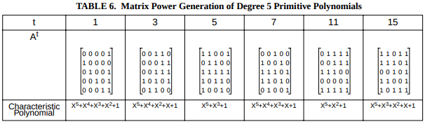
Look at \( \mathbf{A}, \mathbf{A}^3, \mathbf{A}^5 \), and \( \mathbf{A}^7 \). Each time you multiply by \( \mathbf{A} \), the leftmost column disappears and the rightmost column can be obtained from the preceding column by an LFSR update, since the rightmost column is just the coefficients of \( x^{j+(N-1)} \) in the corresponding finite field \( GF(2)[x]/p_1(x) \).
So we don’t need to compute \( \mathbf{A}^j \) with a matrix multiply, which costs \( O(N^3) \) every time we increase \( j \) by 2. Instead, we can just perform a pair of LFSR updates, which cost either \( O(N) \) or \( O(1) \) depending on how strict you are in accounting for computation cost. (If you use fixed-size integers like uint64_t or uint128_t then LFSR update amounts to a shift and conditional XOR in \( O(1) \); if you use an array of bytes to deal with large \( N \) then the LFSR update is \( O(N) \). Of course, the whole idea of big-O notation is to summarize asymptotic behavior as \( N \) becomes very large… but it depends on the typical range of numbers; sometimes \( N=100 \) is very large, and sometimes it isn’t.)
This should shift the bottleneck in execution time to \( O(N^3) \) per primitive polyomial, for the characteristic polynomial calculation. The matrix update is much less significant; at most it is \( O(N) \) cost every time we increase \( j \), and since we do this \( O(N \ln N) \) on average, matrix update cost per primitive polynomial should be at most \( O(N^2 \log N) \).
Let’s do it:
def prim_construct_2(N, p1, maxcount=None):
    """
    Find up to maxcount primitive polynomials of degree N.
    Approach: Compute the characteristic polynomial of
      the jth power of the companion matrix to the first
      primitive polynomial p1(x) we can find, but use
      LFSR updates instead of matrix multiplication.
      Stateful: relies on previous matrix content for speedup.
    """
    m = (1<<N)-1
    A = companion_matrix_with_char_poly(p1)
    Aj = A
    count = 1
    qr = GF2QuotientRing(p1)
    u = qr.lshiftraw(1,N)
    yield 1, p1
    for j in xrange(3,1<<(N-1),2):
        # Update A^j
        Aj = np.roll(Aj,-2,axis=1)
        for c in [-2,-1]:
            u = qr.lshiftraw1(u)
            for i in xrange(N):
                Aj[i,c] = (u >> i) & 1
        if j > smallest_conjugate(j,N):
            continue
        if gcd(j,m) != 1:
            continue
        pj = charpoly_gf2(Aj)
        yield j,pj
        count += 1
        if count == maxcount:
            break

collect_prim_poly(prim_construct_2,8,verbose=True);
j = 1: 11d j = 7: 169 j = 11: 1e7 j = 13: 12b j = 19: 165 j = 23: 163 j = 29: 18d j = 31: 12d j = 37: 15f j = 43: 1c3 j = 47: 1a9 j = 53: 187 j = 59: 14d j = 61: 1cf j = 91: 1f5 j = 127: 171 16 primitive polynomials found
Decimation
We can do the same thing using \( j \) as the decimation ratio for an LFSR. As mentioned in Part IX, this involves two steps:
- creating a decimated output sequence \( {Y_j} = y[0], y[j], y[2j], \ldots, y[(2N-2)j], y[(2N-1)j] \) based on taking every \( j \)th element of the output sequence \( y[k] \) which is the most significant bit of \( x^k \bmod p_1(x) \).
- using the Berlekamp-Massey algorithm to figure out the characteristic polynomial of this sequence.
from libgf2.util import state_from_reversed_output, berlekamp_massey
from libgf2.gf2 import GF2Element

def decimate_LFSR(field, j):
    N = field.degree
    # Construct decimated sequence from the most significant bit (= bit N-1)
    decimated_sequence = [(field.lshiftraw(1,j*k)) >> (N-1) for k in xrange(2*N)]
    # Figure out the minimal polynomial of the decimated sequence
    poly, _ = berlekamp_massey(decimated_sequence)
    return poly

def prim_construct_3(N, p1, maxcount=None):
    """
    Find up to maxcount primitive polynomials of degree N.
    Approach: Find the characteristic polynomial of the LFSR,
      using Berlekamp-Massey, that decimates the output
      of the base LFSR with characteristic polynomial p1(x),
      the first primitive polynomial we can find.
      Stateless; computes a finite field power
      for each bit in the decimated sequence.
    """
    m = (1<<N)-1
    qr = GF2QuotientRing(p1)
    count = 1
    yield 1,p1
    for j in xrange(3,1<<(N-1),2):
        if j > smallest_conjugate(j,N):
            continue
        if gcd(j,m) != 1:
            continue
        pj = decimate_LFSR(qr, j)
        yield j,pj
        count += 1
        if count == maxcount:
            break

collect_prim_poly(prim_construct_3,8,verbose=True);
j = 1: 11d j = 7: 169 j = 11: 1e7 j = 13: 12b j = 19: 165 j = 23: 163 j = 29: 18d j = 31: 12d j = 37: 15f j = 43: 1c3 j = 47: 1a9 j = 53: 187 j = 59: 14d j = 61: 1cf j = 91: 1f5 j = 127: 171 16 primitive polynomials found
This implementation is actually slower than the matrix-based methods. Finding \( x^{k} \bmod p(x) \) involves raising to a power, which takes \( O(N^2 \ln k) \), and if \( k \) is close to \( N \) then we’re talking about \( O(N^3) \). Creating the bit sequence in question requires calculating \( 2N \) of these powers of \( x \), so that’s \( O(N^4) \), and we lose.
But the powers of \( x \) are \( 1, x^j, x^{2j}, x^{3j}, … \) so instead of raising powers each time we need a new term in the bit sequence, we really should only need to raise a power once to compute \( x^j \), and then for each new output bit in the sequence, perform another multiplication by \( x^j \). This would take total of \( O(N^3) \) per primitive polynomial to construct the bit sequence. (\( O(N^3) \) for the initial \( x^j \) calculation performed once, and \( O(N^2) \) per multiply, repeated for each of the \( 2N \) bits.)
Berlekamp-Massey has a worst-case execution time of \( O(N^2) \), so that doesn’t take much computation.
So we should be able to get down to \( O(N^3) \) per primitive polynomial if we restructure the bit sequence calculation:
def LFSR_bit_sequence(field, a, nbits):
    """
    generate the high bit of 1, a, a^2, ...
    """
    u = 1
    for _ in xrange(nbits):
        yield (u >> (field.degree - 1)) & 1
        u = field.mulraw(u,a)

def find_decimated_LFSR_polynomial(field, j):
    uj = field.lshiftraw(1,j)

    decimated_sequence = list(LFSR_bit_sequence(field, uj, 2*field.degree))
    # Return the minimal polynomial of the decimated sequence
    poly, _ = berlekamp_massey(decimated_sequence)
    return poly

def prim_construct_4(N, p1, maxcount=None):
    """
    Find up to maxcount primitive polynomials of degree N.
    Approach: Find the characteristic polynomial of the LFSR,
      using Berlekamp-Massey, that decimates the output
      of the base LFSR with characteristic polynomial p1(x),
      the first primitive polynomial we can find.
      Stateless; computes a single finite field power = x^j
      for each value of j, and a finite field multiply for
      each of 2N bits in the decimated sequence.
    """
    m = (1<<N)-1
    qr = GF2QuotientRing(p1)
    count = 1
    yield 1, p1
    for j in xrange(3,1<<(N-1),2):
        if j > smallest_conjugate(j,N):
            continue
        if gcd(j,m) != 1:
            continue
        pj = find_decimated_LFSR_polynomial(qr, j)
        yield j, pj
        count += 1
        if count == maxcount:
            break

collect_prim_poly(prim_construct_4,8,verbose=True);
j = 1: 11d j = 7: 169 j = 11: 1e7 j = 13: 12b j = 19: 165 j = 23: 163 j = 29: 18d j = 31: 12d j = 37: 15f j = 43: 1c3 j = 47: 1a9 j = 53: 187 j = 59: 14d j = 61: 1cf j = 91: 1f5 j = 127: 171 16 primitive polynomials found
Calculating Minimal Polynomials Directly
There is a way to calculate the minimal polynomial directly; if we have some element \( u=x^j \) in the finite field \( GF(2)[x]/p_1(x) \), then we can compute the polynomial
$$p_j(x) = (x-u)(x-u^2)(x-u^4)\ldots(x-u^{2^{N-1}})$$
The coefficients of this polynomial are always, through the magic of finite fields, 0 or 1, even though they are effectively sums of products of finite field elements. This is straightforward to utilize:
def minimal_polynomial_from_factors(field, u):
    N = field.degree
    p = [1,u]
    # p is our polynomial, starting with (x-u)
    # and we want to calculate (x-u)(x-u^2)(x-u^4)...
    upow = u
    for i in xrange(1,N):
        # invariant at top of loop: degree(p) = i
        upow = field.mulraw(upow,upow)
        # multiply by (x-upow)
        # first multiply by x
        xp = p[:]+[0]
        p = [0]+p
        # then multiply by upow and add
        for j in xrange(i+2):
            p[j] = field.mulraw(p[j],upow) ^ xp[j]
    # p should now be a list of zeros and ones
    pvec = 0
    for i in xrange(N+1):
        assert p[i] == 0 or p[i] == 1
        pvec = (pvec << 1) ^ p[i]
    return pvec

def prim_construct_5(N, p1, maxcount=None):
    """
    Find up to maxcount primitive polynomials of degree N.
    Approach: Find the minimal polynomial of u=x^j directly
    by computing (x-u)(x-u^2)(x-u^4)...(x-u^(2^(N-1))).
    Stateful: steps through odd values of j, updates
    u=x^j by two left shifts each iteration.
    """
    m = (1<<N)-1
    qr = GF2QuotientRing(p1)
    count = 1
    yield 1, p1
    xj = 2
    for j in xrange(3,1<<(N-1),2):
        xj = qr.lshiftraw(xj,2)
        if j > smallest_conjugate(j,N):
            continue
        if gcd(j,m) != 1:
            continue
        pj = minimal_polynomial_from_factors(qr, xj)
        yield j, pj
        count += 1
        if count == maxcount:
            break

collect_prim_poly(prim_construct_5,8,verbose=True);
j = 1: 11d j = 7: 169 j = 11: 1e7 j = 13: 12b j = 19: 165 j = 23: 163 j = 29: 18d j = 31: 12d j = 37: 15f j = 43: 1c3 j = 47: 1a9 j = 53: 187 j = 59: 14d j = 61: 1cf j = 91: 1f5 j = 127: 171 16 primitive polynomials found
Works like a charm. Unfortunately, the minimal polynomial calculation shown here uses a finite field multiplication (\( O(N^2) \)) in a loop that runs \( (N^2+3N-4)/2 \) times, so it looks like it has an overall execution time of \( O(N^4) \) for each primitive polynomial.
Minimal Polynomials using Linear Algebra and Basis Elements
There’s a more efficient method of determining minimal polynomials, if we’re willing to turn to some linear algebra to help. We take \( u = x^j \) and express \( 1, u, u^2, u^3, \ldots, u^{N-1}, u^N \) in terms of the basis \( 1, x, x^2, x^3, \ldots, x^{N-1} \) — which we get for free when we use bit vector representation, since this is the basis we have already been using — and solve for coefficients \( c_i \) that are not all zero, such that \( c_0 + c_1u + c_2u^2 + c_3u^3 + \ldots + c_{N-1}u^{N-1} +c_{N}u^N = 0 \).
For example, suppose we have the example we’ve been using, \( N=8 \) and \( p_1(x) = x^8 + x^4 + x^3 + x^2 + 1 \) with \( j=7 \). Then here are the powers of \( u \):
u = GF2Element(1,0x11d) << 7
for i in xrange(9):
    print "u^%d = %s" % (i, u**i)
u^0 = GF2Element(0b00000001,0x11d) u^1 = GF2Element(0b10000000,0x11d) u^2 = GF2Element(0b00010011,0x11d) u^3 = GF2Element(0b01110101,0x11d) u^4 = GF2Element(0b00011000,0x11d) u^5 = GF2Element(0b10011100,0x11d) u^6 = GF2Element(0b10110101,0x11d) u^7 = GF2Element(0b10001100,0x11d) u^8 = GF2Element(0b01011101,0x11d)
We can see which elements have a 1-bit in their least significant bit, which means that that \( c_0 + c_2 + c_3 + c_6 + c_8 = 0 \). Similarly, if we look at bit 1 of each of these elements, it means that \( c_2 = 0 \). This gives us eight equations with nine unknowns… except that we know that \( c_8 = 1 \) (otherwise it wouldn’t be a primitive polynomial of degree 8) and we can solve it. Essentially we use the \( u^8 \) element to solve \( \mathbf{A}c=u^8 \) where \( \mathbf{A} \) is the matrix formed by the coefficients of \( u^0, u^1, \ldots u^7 \).
For \( j=7 \) we have a specific example of
$$\begin{align} \mathbf{A} &= \begin{bmatrix} 0&0&0&0&0&0&0&1 \cr 1&0&0&0&0&0&0&0 \cr 0&0&0&1&0&0&1&1 \cr 0&1&1&1&0&1&0&1 \cr 0&0&0&1&1&0&0&0 \cr 1&0&0&1&1&1&0&0 \cr 1&0&1&1&0&1&0&1 \cr 1&0&0&0&1&1&0&0 \end{bmatrix}^{HT} \cr u^8 &= \begin{bmatrix}0&1&0&1&1&1&0&1\end{bmatrix}^{HT} \end{align}$$
where the superscript \( H \) refers to a horizontal mirroring, since we want coefficients in ascending order. This equation \( \mathbf{A}c=u^8 \) has solution \( c = \begin{bmatrix}1&0&0&1&0&1&1&0\end{bmatrix}^T \) indicating \( 1 + x^3 + x^5 + x^6 + x^8 \) or 0x169.
A = np.fliplr(np.matrix(
              [[0,0,0,0,0,0,0,1],
               [1,0,0,0,0,0,0,0],
               [0,0,0,1,0,0,1,1],
               [0,1,1,1,0,1,0,1],
               [0,0,0,1,1,0,0,0],
               [1,0,0,1,1,1,0,0],
               [1,0,1,1,0,1,0,1],
               [1,0,0,0,1,1,0,0]])).T
b = np.fliplr(np.matrix(np.array([0,1,0,1,1,1,0,1]))).T
c = np.linalg.solve(A,b).astype(int) & 1
print ("c.T=%s" % c.T)
print ("poly=0x%x" % (sum(ci<<i for i,ci in enumerate(c)) + (1<<len(c))))
c.T=[[1 0 0 1 0 1 1 0]] poly=0x169
We don’t need the numpy library here; we can apply this ourselves from scratch:
def gf2_solve(A,b,N):
    """ Solve Ac=b in mask-encoded form
    A is a list of N bit vectors
    b is a bit vector
    """
    remaining_pivots = [1]*N
    permutation = [0]*N
    for i in xrange(N):
        # Find pivot
        pivot = -1
        mask = 1<<i
        for j in xrange(N):
            if remaining_pivots[j] == 0:
                continue
            if A[j] & mask:
                pivot = j
                break
        if pivot == -1:
            raise ValueError('No solution')
        permutation[i] = pivot
        remaining_pivots[pivot] = 0
        # Eliminate pivot
        for j in xrange(N):
            if j == pivot:
                continue
            if A[j] & mask:
                A[j] ^= A[pivot]
                b ^= ((b >> pivot) & 1) << j
    # Now find solution
    return sum(1<<i for i in xrange(N) if (b >> permutation[i]) & 1)

def minimal_polynomial_from_basis(field, u):
    """ Finds minimal polynomial from basis using linear algebra,
    assuming it is an Nth degree polynomial.
    (If we relax this restriction, this function
    needs to be more complicated, and then we can try lower degree polynomials.)

    This implementation uses Gaussian elimination; by using
    bit masks, we can do the elimination part in O(N^2).
    But the construction of the matrix A requires N finite field multiplications
    for a total of O(N^3).
    """
    N = field.degree
    # Determine u^i from i=0 to i=N (inclusive)
    elements = []
    ui = 1
    for i in xrange(N):
        elements.append(ui)
        ui = field.mulraw(ui, u)
    uN = ui
    # Transpose the element vectors into a matrix of bit masks
    A = [0]*N
    for i in xrange(N):
        mask = 1<<i
        for j in xrange(N):
            if elements[j] & mask:
                A[i] ^= (1<<j)
    c = gf2_solve(A,uN,N)
    c ^= (1<<N)
    # Verify solution
    y = 0
    for i in xrange(N):
        if (c >> i) & 1:
            y ^= elements[i]
    if y != uN:
        raise ValueError("Could not verify solution")
    return c

def prim_construct_6(N, p1, maxcount=None):
    """
    Find up to maxcount primitive polynomials of degree N.
    Approach: Find the minimal polynomial of x^j using linear algebra.
    Stateful: steps through odd values of j, updates
    u=x^j by two left shifts each iteration.
    """
    m = (1<<N)-1
    qr = GF2QuotientRing(p1)
    count = 1
    yield 1, p1
    xj = 2
    for j in xrange(3,1<<(N-1),2):
        xj = qr.lshiftraw(xj,2)
        if j > smallest_conjugate(j,N):
            continue
        if gcd(j,m) != 1:
            continue
        pj = minimal_polynomial_from_basis(qr, xj)
        yield j, pj
        count += 1
        if count == maxcount:
            break

collect_prim_poly(prim_construct_6,8,verbose=True);
j = 1: 11d j = 7: 169 j = 11: 1e7 j = 13: 12b j = 19: 165 j = 23: 163 j = 29: 18d j = 31: 12d j = 37: 15f j = 43: 1c3 j = 47: 1a9 j = 53: 187 j = 59: 14d j = 61: 1cf j = 91: 1f5 j = 127: 171 16 primitive polynomials found
Other Approaches
If we turn to the authoritative references on LFSRs and finite fields, we see this advice:
-
Golomb’s Shift Register Sequences: Golomb devotes a full section (“Computational Techniques”) on identifying primitive polynomials. The sieve methods discussed are more or less the same as Saxena and McCluskey’s FactorPower. For the synthetic method, Golomb mentions a “superposition of cosets” approach to find all the primitive polynomials, something to do with computing a matrix of coefficients relating the canonical shift register sequences (shifted so that \( a[k] = a[2^wk] \), that is, the sequence is invariant to decimations of powers of two) to each of the corresponding cyclotomic cosets — which doesn’t make any sense to me, first because I don’t understand it completely (Golomb’s writing is cryptic and vague at times, leaving the reader to guess the implication of some informally-stated hint), and second, because the number of cosets increases as \( \varphi(2^N-1) \sim O(2^N/(N \ln N)) \), so even if you want to find just a handful of primitive polynomials, you have to incur the up-front cost of doing something once for each primitive polynomial you might generate later.
-
McEliece’s Finite Fields for Computer Scientists and Engineers: McEliece has one chapter on \( m \)-sequences and shows that any maximal-length LFSR sequence of a given degree can be derived from any other of the same degree, by decimation.
-
Lidl & Niederreiter’s Introduction to Finite Fields and Their Applications: There is one section called “Construction of Irreducible Polynomials” that cites three synthetic methods:
- computing \( p_j(x) \) such that \( p_j(x^j) = \prod\limits_{i=1}^jp_1(\omega_ix) \) where \( \omega_i \) is one of the \( j \)th roots of unity — this doesn’t seem to translate so well into an efficient computation technique
- computing characteristic polynomials of powers of the companion matrix, as we’ve already seen
- computing minimal polynomials, as we’ve already seen
-
John Kerl’s Computation in Finite Fields: While sections of Kerl’s document are gloriously in-depth and easy to follow, he spends three paragraphs outlining a sieve approach for checking primitivity before going on to another topic.
Other papers:
- Živković describes a sieve method optimized for finding primitive polynomials with a low coefficient count \( t \)
- Mitra describes a sieve method, but it requires \( O(2^N) \) computation time, so it seems poorly thought-out
- Di Porto, Guida, and Montolivo describe a synthetic method using LFSR decimation and the Berlekamp-Massey algorithm. There is a twist to it to speed things up, however. I call this the St. Ives Algorithm, and I’ll describe it in more detail below.
- Gordon describes a synthetic technique for calculating the minimal polynomial directly.
- Shoup describes a clever synthetic technique, also using LFSR decimation and the Berlekamp-Massey algorithm, but it is totally different, and, once again, I’ll describe it below.
We Can Do Better!
There are four improvements for synthetic methods, which are minor variations, but they all accomplish key improvements. Three of them are based around methods using the Berlekamp-Massey algorithm to process decimations of an LFSR bit sequence. The fourth, Gordon’s method uses an insight for making it easy to compute the minimal polynomial directly.
The St. Ives Algorithm
The problem with using decimation and Berlekamp-Massey is that it takes so long to construct bit sequences as input to Berlekamp-Massey. In prim_construct_4() we came up with an optimization where we computed \( 1, x^j, x^{2j}, x^{3j}, \ldots, x^{(2N-1)j} \) as repeated finite field multiplications of \( x^j \). Each multiplication takes \( O(N^2) \) operations, and since we do this \( 2N-1 \) times, constructing the whole bit sequences takes \( O(N^3) \).
I thought about that while writing this article. We lowered the runtime by reducing the required operation from a raise-to-the-power, to a multiply. Maybe we could do something similar, and reduce the required operation from a multiply to an LFSR update, which takes (depending on how nitpicky you are) either \( O(1) \) or \( O(N) \) execution time? We could, for example, compute \( x^j \) by starting with 1 and performing \( j \) LFSR updates, then computing \( x^{2j} \) with another \( j \) LFSR updates, and so on, completing the entire required bit sequence after \( (2N-1)j \) updates — this is either \( O(jN) \) or \( O(jN^2) \) operations, depending on how you define things. The only problem is that it takes longer if \( j \) is large. But that’s not a big deal. We just need to find the smallest value of \( j \) that is relatively prime to \( 2^N-1 \):
candidates = [3,5,7,11,13,17,19,23,29]
for N in xrange(2,33):
    m = (1<<N) - 1
    for j in candidates:
        if gcd(j,m) == 1:
            print "N=%2d, j=%d" % (N,j)
            break
    else:
        print "N=%2d, j>30 (UH OH!)" % N
N= 2, j=5 N= 3, j=3 N= 4, j=7 N= 5, j=3 N= 6, j=5 N= 7, j=3 N= 8, j=7 N= 9, j=3 N=10, j=5 N=11, j=3 N=12, j=11 N=13, j=3 N=14, j=5 N=15, j=3 N=16, j=7 N=17, j=3 N=18, j=5 N=19, j=3 N=20, j=7 N=21, j=3 N=22, j=5 N=23, j=3 N=24, j=11 N=25, j=3 N=26, j=5 N=27, j=3 N=28, j=7 N=29, j=3 N=30, j=5 N=31, j=3 N=32, j=7
Most of the time, in fact whenever \( N \) is odd, we can get away with \( j=3 \). If \( N \) is even, then \( j \) is at least \( 5 \). If \( N \) is a multiple of 4, then \( j \) is at least 7. (But \( j=7 \) suffices for all powers of 2.) If \( N \) is a multiple of 12, then \( j \) is at least 11. It is very rare to need more than \( j=11 \):
candidates = [3,5,7,11,13,17,19,23,29]
for N in xrange(2,2000):
    m = (1<<N) - 1
    for j in candidates:
        if gcd(j,m) == 1:
            if j > 11:
                print "N=%2d, j=%d" % (N,j)
            break
    else:
        print "N=%2d, j>30 (UH OH!)" % N
N=60, j=17 N=120, j=19 N=180, j=17 N=240, j=19 N=300, j=17 N=360, j=23 N=420, j=17 N=480, j=19 N=540, j=17 N=600, j=19 N=660, j=17 N=720, j=23 N=780, j=17 N=840, j=19 N=900, j=17 N=960, j=19 N=1020, j=17 N=1080, j=23 N=1140, j=17 N=1200, j=19 N=1260, j=17 N=1320, j=19 N=1380, j=17 N=1440, j=23 N=1500, j=17 N=1560, j=19 N=1620, j=17 N=1680, j=19 N=1740, j=17 N=1800, j=23 N=1860, j=17 N=1920, j=19 N=1980, j=17
It’s only the multiples of 60 where you need \( j\ge 17 \), and the multiples of 360 where you need \( j \ge 23 \), and the multiples of 3960 where you need \( j\ge 29 \). I’m unlikely to ever use \( N > 64 \), so \( j=17 \) suffices for all small values.
So that’s fine and dandy, but what happens when we need more than 2 primitive polynomials? The first one we had to get from a sieve method (or from someone else’s work in a table), and the second we could use this approach of decimating by a small \( j \) and then using Berlekamp-Massey, but what happens as we need to increase \( j \)? For \( N=8 \) the required sequence of \( j \) values was \( 1,7,11,13,19,23,29,31,37,43,47,53,59,61,91,127 \), and with larger values of \( N \) the maximum \( j \) value will be \( 2^{N-1} - 1 \), which is not small.
The key here is to look at \( j \) as a possible generator in the multiplicative group \( \bmod 2^N-1 \) of integers relatively prime to \( 2^N-1 \):
N = 8
j0 = 7
m = (1<<N) - 1
j = 1
for i in xrange(16):
    print("j = %d^%2d mod 255 = %3d -> smallest conjugate %d" %
          (j0, i, j, smallest_conjugate(j,N)))
    j = (j * j0) % m
j = 7^ 0 mod 255 = 1 -> smallest conjugate 1 j = 7^ 1 mod 255 = 7 -> smallest conjugate 7 j = 7^ 2 mod 255 = 49 -> smallest conjugate 19 j = 7^ 3 mod 255 = 88 -> smallest conjugate 11 j = 7^ 4 mod 255 = 106 -> smallest conjugate 53 j = 7^ 5 mod 255 = 232 -> smallest conjugate 29 j = 7^ 6 mod 255 = 94 -> smallest conjugate 47 j = 7^ 7 mod 255 = 148 -> smallest conjugate 37 j = 7^ 8 mod 255 = 16 -> smallest conjugate 1 j = 7^ 9 mod 255 = 112 -> smallest conjugate 7 j = 7^10 mod 255 = 19 -> smallest conjugate 19 j = 7^11 mod 255 = 133 -> smallest conjugate 11 j = 7^12 mod 255 = 166 -> smallest conjugate 53 j = 7^13 mod 255 = 142 -> smallest conjugate 29 j = 7^14 mod 255 = 229 -> smallest conjugate 47 j = 7^15 mod 255 = 73 -> smallest conjugate 37
That generated half of the values we need. What about the other ones? We find the smallest factor not used yet, which is 13 in this case, and use it:
N = 8
j0 = 7
j1 = 13
m = (1<<N) - 1
j = 1
i0 = 0
i1 = 0
for i in xrange(16):
    c = smallest_conjugate(j,N)
    if i > 1 and c == 1:
        i1 += 1
        j = (j * j1) % m
        c = smallest_conjugate(j,N)
    print("j = (%d^%2d)*(%d^%2d) mod 255 = %3d -> smallest conjugate %d" %
          (j0, i0, j1, i1, j, c))
    j = (j * j0) % m
    i0 += 1
j = (7^ 0)*(13^ 0) mod 255 = 1 -> smallest conjugate 1 j = (7^ 1)*(13^ 0) mod 255 = 7 -> smallest conjugate 7 j = (7^ 2)*(13^ 0) mod 255 = 49 -> smallest conjugate 19 j = (7^ 3)*(13^ 0) mod 255 = 88 -> smallest conjugate 11 j = (7^ 4)*(13^ 0) mod 255 = 106 -> smallest conjugate 53 j = (7^ 5)*(13^ 0) mod 255 = 232 -> smallest conjugate 29 j = (7^ 6)*(13^ 0) mod 255 = 94 -> smallest conjugate 47 j = (7^ 7)*(13^ 0) mod 255 = 148 -> smallest conjugate 37 j = (7^ 8)*(13^ 1) mod 255 = 208 -> smallest conjugate 13 j = (7^ 9)*(13^ 1) mod 255 = 181 -> smallest conjugate 91 j = (7^10)*(13^ 1) mod 255 = 247 -> smallest conjugate 127 j = (7^11)*(13^ 1) mod 255 = 199 -> smallest conjugate 31 j = (7^12)*(13^ 1) mod 255 = 118 -> smallest conjugate 59 j = (7^13)*(13^ 1) mod 255 = 61 -> smallest conjugate 61 j = (7^14)*(13^ 1) mod 255 = 172 -> smallest conjugate 43 j = (7^15)*(13^ 1) mod 255 = 184 -> smallest conjugate 23
The reason I call it the St. Ives Algorithm is that if \( N \ge 4 \) is a power of 2, \( j \) ends up being powers of 7, just like the nursery rhyme, As I Was Going to St. Ives.
I was disappointed to find out that Di Porto, Guida, and Montolivo already came up with this approach in their 1992 paper, and even more disappointed to find out that you can’t just rely on one value of \( j \), as we saw above. There doesn’t appear to be an easy way to generalize this approach for arbitrary \( N \), which we have seen above, and Di Porto et al don’t discuss a way to work around this limitation if you want to generate all the primitive polynomials.
So I’ve tried to find a way myself.
There is a way to “help” manually if you know the generating set of the multiplicative group \( \bmod 2^N-1 \) of integers relatively prime to \( 2^N-1 \). If we can give a plan of what operations to perform, then maybe we can find all the primitive polynomials.
def multiplicative_plan(generators, N):
    m = (1<<N) - 1
    v = 1
    vc = 1
    ngen = len(generators)
    progress = [0]*ngen
    count = 0
    while count < 100:
        count += 1
        for k in xrange(ngen):
            j,nj = generators[k]
            progress[k] += 1
            vnext = (v*j) % m
            vcnext = smallest_conjugate(vnext, N)
            yield k, j, vc, v
            v = vnext
            vc = vcnext
            if progress[k] < nj:
                break
            progress[k] = 0
        else:
            break

print "k  j  vc   v"
for k,a,jc,j in multiplicative_plan([(7,8),(13,2)], 8):
    print "%d %2d %3d %3d" % (k,a,jc,j)
k j vc v 0 7 1 1 0 7 7 7 0 7 19 49 0 7 11 88 0 7 53 106 0 7 29 232 0 7 47 94 0 7 37 148 1 13 1 16 0 7 13 208 0 7 91 181 0 7 127 247 0 7 31 199 0 7 59 118 0 7 61 61 0 7 43 172 0 7 23 184 1 13 13 13
In the table above, at each step:
- \( k= \) index into the generating set to use
- \( j= \) the corresponding element in the generating set
- \( v= \) the effective decimation ratio: at each step, \( v \leftarrow vj \bmod 2^N-1 \)
- \( v_c= \) the “canonical” value of \( v \) (minimum conjugate under bit rotation)
Of course, it may be difficult to find such a generating set in advance. Here’s an attempt at finding a generating set as we go. The idea is the following:
- Compute \( R = \varphi(2^N-1) \) which is the order of the multiplicative group mod \( 2^N-1 \) of integers relatively prime to \( 2^N-1 \).
- Set \( r=R/N \) which is the number of distinct values under cyclic bit rotation, and which is also the number of primitive polynomials of degree \( N \).
- Create a list \( L \) of low-value odd primes \( 3,5,7,\ldots,p_{max}. \) (\( p_{max}=997 \) might work.)
- Remove all divisors of \( 2^N-1 \) from \( L \).
- Create an empty list \( J \).
- Output the tuple \( (1,0,1) \).
- Set \( v = 1, s=1, n=0. \) The value of \( v \) will be the decimating ratio used at each step; the value of s will be the order of the group generated by elements of \( J \) and the number of values that have been output so far; the value of n will be the size of \( J \).
- Set \( j = \) the lowest remaining element of \( L \).
- Set \( n \leftarrow n+1. \)
- Set \( (v,r_j) = \operatorname{ITERATE}(v,J,L,j,0,n-1,j) \).
- Add the pair \( (j,r_j) \) to the list \( J \).
- Set \( s \leftarrow r_js \)
- If \( s < r \) goto step 8, otherwise we are done, and we should have \( s = r \). (If not, we’ve made a mistake.)
The ITERATE algorithm works as follows, given values \( v,J,L,j,r_j,n,j_{top} \); the value \( r_j \) is either zero (and we have to figure out how many times to multiply by \( j \) until some power of two is reachable) or greater than 1 and we need to multiply by \( j \) that many times.
- Set \( t = 0 \) if \( j=j_{top} \), otherwise set \( t=-1 \). (This makes the algorithm iterate one fewer time at the top level, since previous top-level calls to iterate have already executed; \( v \) should be equal to \( {j_0}^{0}{j_1}^{r_1-1}{j_2}^{r_2-1}\ldots \) at this point.)
- Set \( w=0 \)
- Set \( v \leftarrow jv \bmod 2^N-1 \)
- Set \( t \leftarrow t+1 \)
- If \( n > 0 \), goto step 11
- (\( n=0 \)) Output the tuple \( (v,j,1) \)
- Compute \( v’= \) the smallest bit rotation of \( v \), and remove it from \( L \) if present
- If \( r_j > 0 \) and \( j_{top}v \bmod 2^N-1 \) is a power of two, set \( w=1 \)
- If \( r_j = 0 \) and \( v’ = 1 \) then return \( (v,t) \)
- If \( t < r_j \) then goto step 3
- Otherwise return \( (v,w) \)
- (\( n>0 \)) Output the tuple \( (v,j,0) \)
- Set \( (v,w_{sub}) = \operatorname{ITERATE}(v,J,L,J[n-1][0],J[n-1][1],j_{top}) \)
- If \( w_{sub} = 1 \) then set \( w \leftarrow 1 \)
- If \( t < r_j \) then goto step 2
- If \( t = r_j \) then return \( (v,w) \)
- If \( w = 0 \) then goto step 2
- Otherwise return \( (v,t) \)
The idea here is that we have some number of multipliers \( j_0, j_1, \ldots j_{n-1} \) and each of them has a loop count \( r_0, r_1, \ldots r_{n-1} \). The topmost multiplier \( j_{top} = j_{n-1} \) we need to figure out \( r_{n-1} \) and we pass in 0, looping until the \( n=0 \) level would reach 1 on the next cycle of the topmost multiplier, whereupon we set \( w=1 \) to indicate that this is to be the last outer cycle. The routine returns two numbers; \( v \) is its updated value, and we either return \( w \) (for lower levels) or the cycle count \( t \) for the outermost level.
The output tuple consists of \( v \), the multiplier \( j \) at each step, and a “usage” bit \( u \); if \( u \) is 1 then the resulting value of \( v \) should be used to find an appropriate primitive polynomial, otherwise it should be skipped.
I couldn’t think of a clean way to handle the fact that there is both an “output” and a “return value” in the algorithm above. In Python, at first I tried to yield the output and return the return value, but Python won’t let you do both, so I had to rewrite it a little bit. Here is a Python implementation:
def yield_primitive_polynomial_search_plan(N,J=None):
    factors = factorize_mersenne_candidate(N)
    phi = 1
    for k,v in factors.iteritems():
        phi *= k**(v-1) * (k-1)
    #print "phi=%d,phi/N=%d" % (phi, phi//N)
    def primes_up_to(N):
        L = [3,5,7,11]
        pmin = L[-1]+2
        while pmin<N:
            pmax = min(L[-1]**2, N+1)
            for p in xrange(pmin,pmax,2):
                isprime = True
                for d in L:
                    if d*d > p:
                        break
                    if p % d == 0:
                        isprime = False
                        break
                if isprime:
                    L.append(p)
            pmin = p+2
        return L

    M = (1<<N)-1
    Np = 1000
    L = set(primes_up_to(Np))
    for k in factors:
        if k < Np:
            L.remove(k)
    if J is None:
        J = []

    def iterate(v,j,rj,n,jtop):
        t=0 if j == jtop else -1
        w=0
        while rj == 0 or (t+1)<rj:
            v = (v*j)%M
            t += 1
            if n == 0:
                if rj > 0:
                    vnext = (v*jtop)%M
                    if (vnext & (vnext-1)) == 0:   # power of 2
                        w = 1
                vc = smallest_conjugate(v,N)
                if vc < Np:
                    L.discard(vc)
                if rj > 0:
                    if t >= rj:
                        yield (v,j,0,w)
                        break
                else: # rj == 0
                    if vc == 1:
                        break
                yield (v,j,1,w)
            else:  # n > 0
                if rj == 0 and w == 1:
                    break
                if rj > 0 and t >= rj:
                    break
                yield (v,j,0,w)
                for y in iterate(v,J[n-1][0],J[n-1][1],n-1,jtop):
                    v,_,_,wsub = y
                    w = wsub | w
                    yield y

    s = 1
    v = 1
    yield (1,0,1,0)
    n = 0
    while s*N < phi:
        span = s
        n += 1
        Lmin = min(L)
        J.append((Lmin,0))
        for y in iterate(v,Lmin,0,n-1,Lmin):
            v,j,v_use,w = y
            s += v_use
            yield y
        t = s//span
        J[-1] = (Lmin,t)
        #print "s=%d, j=%d, t=%d" % (s,Lmin,t)
    #print "jdict=%s,J=%s" % (jdict,J)
def show_primitive_polynomial_search_plan(N,smax=3000):
print "Primitive polynomial search plan, N=%d" % N
s=0
s_use = 0
jdict = {}
for y in yield_primitive_polynomial_search_plan(N):
s+=1
if s > smax:
break
v,j,u,w = y
s_use += u
if j > 0:
jdict[j] = jdict.get(j,0) + 1
print("s=%3d su=%3d v=%5d j=%2d u=%d w=%d vc=%5d %s"
% (s,s_use,v,j,u,w, smallest_conjugate(v,N), jdict))
show_primitive_polynomial_search_plan(8)
show_primitive_polynomial_search_plan(9)Primitive polynomial search plan, N=8
s= 1 su= 1 v= 1 j= 0 u=1 w=0 vc= 1 {}
s= 2 su= 2 v= 7 j= 7 u=1 w=0 vc= 7 {7: 1}
s= 3 su= 3 v= 49 j= 7 u=1 w=0 vc= 19 {7: 2}
s= 4 su= 4 v= 88 j= 7 u=1 w=0 vc= 11 {7: 3}
s= 5 su= 5 v= 106 j= 7 u=1 w=0 vc= 53 {7: 4}
s= 6 su= 6 v= 232 j= 7 u=1 w=0 vc= 29 {7: 5}
s= 7 su= 7 v= 94 j= 7 u=1 w=0 vc= 47 {7: 6}
s= 8 su= 8 v= 148 j= 7 u=1 w=0 vc= 37 {7: 7}
s= 9 su= 8 v= 139 j=13 u=0 w=0 vc= 23 {13: 1, 7: 7}
s= 10 su= 9 v= 208 j= 7 u=1 w=0 vc= 13 {13: 1, 7: 8}
s= 11 su= 10 v= 181 j= 7 u=1 w=0 vc= 91 {13: 1, 7: 9}
s= 12 su= 11 v= 247 j= 7 u=1 w=0 vc= 127 {13: 1, 7: 10}
s= 13 su= 12 v= 199 j= 7 u=1 w=0 vc= 31 {13: 1, 7: 11}
s= 14 su= 13 v= 118 j= 7 u=1 w=1 vc= 59 {13: 1, 7: 12}
s= 15 su= 14 v= 61 j= 7 u=1 w=1 vc= 61 {13: 1, 7: 13}
s= 16 su= 15 v= 172 j= 7 u=1 w=1 vc= 43 {13: 1, 7: 14}
s= 17 su= 16 v= 184 j= 7 u=1 w=1 vc= 23 {13: 1, 7: 15}
Primitive polynomial search plan, N=9
s= 1 su= 1 v= 1 j= 0 u=1 w=0 vc= 1 {}
s= 2 su= 2 v= 3 j= 3 u=1 w=0 vc= 3 {3: 1}
s= 3 su= 3 v= 9 j= 3 u=1 w=0 vc= 9 {3: 2}
s= 4 su= 4 v= 27 j= 3 u=1 w=0 vc= 27 {3: 3}
s= 5 su= 5 v= 81 j= 3 u=1 w=0 vc= 37 {3: 4}
s= 6 su= 6 v= 243 j= 3 u=1 w=0 vc= 111 {3: 5}
s= 7 su= 7 v= 218 j= 3 u=1 w=0 vc= 109 {3: 6}
s= 8 su= 8 v= 143 j= 3 u=1 w=0 vc= 61 {3: 7}
s= 9 su= 9 v= 429 j= 3 u=1 w=0 vc= 183 {3: 8}
s= 10 su= 10 v= 265 j= 3 u=1 w=0 vc= 19 {3: 9}
s= 11 su= 11 v= 284 j= 3 u=1 w=0 vc= 57 {3: 10}
s= 12 su= 12 v= 341 j= 3 u=1 w=0 vc= 171 {3: 11}
s= 13 su= 12 v= 172 j= 5 u=0 w=0 vc= 43 {3: 11, 5: 1}
s= 14 su= 13 v= 5 j= 3 u=1 w=0 vc= 5 {3: 12, 5: 1}
s= 15 su= 14 v= 15 j= 3 u=1 w=0 vc= 15 {3: 13, 5: 1}
s= 16 su= 15 v= 45 j= 3 u=1 w=0 vc= 45 {3: 14, 5: 1}
s= 17 su= 16 v= 135 j= 3 u=1 w=0 vc= 29 {3: 15, 5: 1}
s= 18 su= 17 v= 405 j= 3 u=1 w=0 vc= 87 {3: 16, 5: 1}
s= 19 su= 18 v= 193 j= 3 u=1 w=0 vc= 11 {3: 17, 5: 1}
s= 20 su= 19 v= 68 j= 3 u=1 w=0 vc= 17 {3: 18, 5: 1}
s= 21 su= 20 v= 204 j= 3 u=1 w=0 vc= 51 {3: 19, 5: 1}
s= 22 su= 21 v= 101 j= 3 u=1 w=0 vc= 83 {3: 20, 5: 1}
s= 23 su= 22 v= 303 j= 3 u=1 w=0 vc= 95 {3: 21, 5: 1}
s= 24 su= 23 v= 398 j= 3 u=1 w=0 vc= 59 {3: 22, 5: 1}
s= 25 su= 24 v= 172 j= 3 u=1 w=0 vc= 43 {3: 23, 5: 1}
s= 26 su= 24 v= 349 j= 5 u=0 w=0 vc= 187 {3: 23, 5: 2}
s= 27 su= 25 v= 25 j= 3 u=1 w=0 vc= 25 {3: 24, 5: 2}
s= 28 su= 26 v= 75 j= 3 u=1 w=0 vc= 75 {3: 25, 5: 2}
s= 29 su= 27 v= 225 j= 3 u=1 w=0 vc= 23 {3: 26, 5: 2}
s= 30 su= 28 v= 164 j= 3 u=1 w=0 vc= 41 {3: 27, 5: 2}
s= 31 su= 29 v= 492 j= 3 u=1 w=0 vc= 123 {3: 28, 5: 2}
s= 32 su= 30 v= 454 j= 3 u=1 w=0 vc= 55 {3: 29, 5: 2}
s= 33 su= 31 v= 340 j= 3 u=1 w=0 vc= 85 {3: 30, 5: 2}
s= 34 su= 32 v= 509 j= 3 u=1 w=0 vc= 255 {3: 31, 5: 2}
s= 35 su= 33 v= 505 j= 3 u=1 w=0 vc= 127 {3: 32, 5: 2}
s= 36 su= 34 v= 493 j= 3 u=1 w=0 vc= 223 {3: 33, 5: 2}
s= 37 su= 35 v= 457 j= 3 u=1 w=0 vc= 79 {3: 34, 5: 2}
s= 38 su= 36 v= 349 j= 3 u=1 w=0 vc= 187 {3: 35, 5: 2}
s= 39 su= 36 v= 212 j= 5 u=0 w=0 vc= 53 {3: 35, 5: 3}
s= 40 su= 37 v= 125 j= 3 u=1 w=0 vc= 125 {3: 36, 5: 3}
s= 41 su= 38 v= 375 j= 3 u=1 w=0 vc= 239 {3: 37, 5: 3}
s= 42 su= 39 v= 103 j= 3 u=1 w=1 vc= 103 {3: 38, 5: 3}
s= 43 su= 40 v= 309 j= 3 u=1 w=1 vc= 107 {3: 39, 5: 3}
s= 44 su= 41 v= 416 j= 3 u=1 w=1 vc= 13 {3: 40, 5: 3}
s= 45 su= 42 v= 226 j= 3 u=1 w=1 vc= 39 {3: 41, 5: 3}
s= 46 su= 43 v= 167 j= 3 u=1 w=1 vc= 117 {3: 42, 5: 3}
s= 47 su= 44 v= 501 j= 3 u=1 w=1 vc= 191 {3: 43, 5: 3}
s= 48 su= 45 v= 481 j= 3 u=1 w=1 vc= 31 {3: 44, 5: 3}
s= 49 su= 46 v= 421 j= 3 u=1 w=1 vc= 93 {3: 45, 5: 3}
s= 50 su= 47 v= 241 j= 3 u=1 w=1 vc= 47 {3: 46, 5: 3}
s= 51 su= 48 v= 212 j= 3 u=1 w=1 vc= 53 {3: 47, 5: 3}
This effectively forms a path through a lattice structure, with one dimension for each element in the generating set. Here is the resulting path for \( N=8 \):
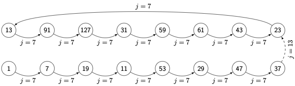
Here the dotted line for \( j=13 \) represents a transition that is skipped for the purpose of determining a primitive polynomial; the resulting value (in this case, decimation ratio 23) will be picked up later in the sequence.
A complete picture of all the \( j=7 \) and \( j=13 \) transitions within this multiplicative group is shown below, with solid lines denoting multiplication by \( j=7 \) and dashed lines denoting multiplication by \( j=13 \):
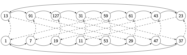
You can see here that \( j=7 \) has order 8 (it takes 8 transitions to get through a cycle) and \( j=13 \) has order 4 (example: the cycle, 1, 13, 53, 59) but they are not completely orthogonal, since multiplication by \( j=13 \) zigzags back and forth between the two cosets (the lower and upper cycles of \( j=7 \)).
I have no idea how experienced mathematicians visualize noncyclic groups; this is a relatively simple one and yet it’s very busy even showing the cycles generated by two of its elements.
At any rate, this method seems to work well; I’ve run it on a bunch of different values of \( N \), including complete runs up to \( N=25 \), and it seems to find a generating set of small primes for all the complete runs. (The optional J parameter gets filled in by pairs \( (j,r_j) \) which are the decimation ratio multiplier \( j \) and its run length \( r_j \); the value of \( r_j \) is initialized to 0 and corrected later once a complete cycle is achieved for the elements of the generating set identified so far. For example, with \( N=25 \) we can use \( j=3 \) to get a cycle of 450 primitive polynomials and \( j=\{3,5\} \) to get a cycle of \( 450 \times 60 = 27000 \) primitive polynomials; \( j=\{3,5,7\} \) bumps it up to 648000, and \( j=\{3,5,7,11\} \) reaches the full set of 1296000 primitive polynomials for \( N=25 \).)
for N in xrange(3,64):
    su = 0
    J=[]
    for y in yield_primitive_polynomial_search_plan(N,J):
        su += y[2]
        nmax = 1300000 if N <= 25 else 25000
        if su >= nmax:
            break
    print "N=%d, su=%d, J=%s" % (N,su,J)
N=3, su=2, J=[(3, 2)] N=4, su=2, J=[(7, 2)] N=5, su=6, J=[(3, 6)] N=6, su=6, J=[(5, 6)] N=7, su=18, J=[(3, 18)] N=8, su=16, J=[(7, 8), (13, 2)] N=9, su=48, J=[(3, 12), (5, 4)] N=10, su=60, J=[(5, 30), (13, 2)] N=11, su=176, J=[(3, 88), (5, 2)] N=12, su=144, J=[(11, 12), (17, 6), (23, 2)] N=13, su=630, J=[(3, 70), (5, 3), (7, 3)] N=14, su=756, J=[(5, 42), (7, 18)] N=15, su=1800, J=[(3, 150), (5, 6), (11, 2)] N=16, su=2048, J=[(7, 128), (11, 8), (13, 2)] N=17, su=7710, J=[(3, 7710)] N=18, su=7776, J=[(5, 72), (11, 18), (17, 3), (23, 2)] N=19, su=27594, J=[(3, 27594)] N=20, su=24000, J=[(7, 120), (13, 10), (17, 10), (19, 2)] N=21, su=84672, J=[(3, 504), (5, 84), (13, 2)] N=22, su=120032, J=[(5, 1364), (7, 44), (19, 2)] N=23, su=356960, J=[(3, 178480), (5, 2)] N=24, su=276480, J=[(11, 24), (19, 48), (23, 10), (29, 2), (31, 2), (37, 6)] N=25, su=1296000, J=[(3, 450), (5, 60), (7, 24), (11, 2)] N=26, su=25000, J=[(5, 2730), (7, 0)] N=27, su=25000, J=[(3, 14592), (5, 0)] N=28, su=25000, J=[(7, 252), (11, 0)] N=29, su=25000, J=[(3, 0)] N=30, su=25000, J=[(5, 1650), (13, 0)] N=31, su=25000, J=[(3, 0)] N=32, su=25000, J=[(7, 0)] N=33, su=25000, J=[(3, 0)] N=34, su=25000, J=[(5, 0)] N=35, su=25000, J=[(3, 0)] N=36, su=25000, J=[(11, 216), (17, 36), (23, 0)] N=37, su=25000, J=[(3, 0)] N=38, su=25000, J=[(5, 0)] N=39, su=25000, J=[(3, 0)] N=40, su=25000, J=[(7, 0)] N=41, su=25000, J=[(3, 0)] N=42, su=25000, J=[(5, 0)] N=43, su=25000, J=[(3, 0)] N=44, su=25000, J=[(7, 0)] N=45, su=25000, J=[(3, 0)] N=46, su=25000, J=[(5, 0)] N=47, su=25000, J=[(3, 0)] N=48, su=25000, J=[(11, 1344), (19, 0)] N=49, su=25000, J=[(3, 0)] N=50, su=25000, J=[(5, 8100), (7, 0)] N=51, su=25000, J=[(3, 0)] N=52, su=25000, J=[(7, 0)] N=53, su=25000, J=[(3, 0)] N=54, su=25000, J=[(5, 0)] N=55, su=25000, J=[(3, 0)] N=56, su=25000, J=[(7, 0)] N=57, su=25000, J=[(3, 0)] N=58, su=25000, J=[(5, 0)] N=59, su=25000, J=[(3, 0)] N=60, su=25000, J=[(17, 6600), (19, 0)] N=61, su=25000, J=[(3, 0)] N=62, su=25000, J=[(5, 0)] N=63, su=25000, J=[(3, 0)]
Okay, but we haven’t actually found any primitive polynomials yet. We’ve just been finding decimation ratios that cover the full set. In order to find the polynomials themselves we have to take LFSR samples and run them through Berlekamp-Massey. Remember, the St. Ives algorithm collects \( j(2N-1) + 1 \) samples total, so for \( N=8 \) and \( j=7 \) we need to generate bits \( b[0] \) through \( b[105] \) and retain samples \( b[0], b[7], b[14], b[21], b[28], b[35], b[42], \ldots, b[98], b[105] \) to feed into Berlekamp-Massey.
The usage bit output from the search plan algorithm just tells you whether the new decimation ratio produces a primitive polynomial that we should report; we still have to run Berlekamp-Massey so that we have a new primitive polynomial for the following decimation ratio.
Let’s do it!
def prim_construct_st_ives(N,p1,maxcount=None):
    """
    Implement the St. Ives algorithm
    (Di Porto, Guida, and Montolivo, by computing 1+(2N-1)j bits
    in order to decimate by a small ratio j, varying j when necessary)
    Stateful: depends on previous polynomial each time.
    """
    qr = GF2QuotientRing(p1)
    poly= p1
    count = 0
    for v,j,usage_bit,w in yield_primitive_polynomial_search_plan(N):
        if j == 0:
            # we get this the very beginning;
            # just output the original polynomial
            yield v,poly
            count += 1
            continue
        # Generate enough bits in the LFSR output sequence,
        # decimated by j
        e = 1
        bits = [0]
        for _ in xrange(2*N-1):
            for i in xrange(j):
                e = qr.lshiftraw1(e)
            bits.append(e>>(N-1))
        poly,N_expected = berlekamp_massey(bits)
        qr = GF2QuotientRing(poly)

        # Only report the polynomial if the usage bit is 1
        if usage_bit:
            yield v,poly
            count += 1
            if count == maxcount:
                break

st_ives_polynomials = sorted(collect_prim_poly(
                              prim_construct_st_ives, 8, verbose=True))
prim_construct_1_polynomials = sorted(collect_prim_poly(
                              prim_construct_1, 8))

print st_ives_polynomials
print prim_construct_1_polynomials
print("Match? "+("YES"
                if st_ives_polynomials == prim_construct_1_polynomials
                else "NO"))
j = 1: 11d j = 7: 169 j = 49: 165 j = 88: 1e7 j = 106: 187 j = 232: 18d j = 94: 1a9 j = 148: 15f j = 208: 12b j = 181: 1f5 j = 247: 171 j = 199: 12d j = 118: 14d j = 61: 1cf j = 172: 1c3 j = 184: 163 16 primitive polynomials found [285, 299, 301, 333, 351, 355, 357, 361, 369, 391, 397, 425, 451, 463, 487, 501] [285, 299, 301, 333, 351, 355, 357, 361, 369, 391, 397, 425, 451, 463, 487, 501] Match? YES
Ho hum, it’s kind of boring when things work out correctly.
Just for kicks, let’s try it on \( N=20 \), which should generate 24000 different primitive polynomials, and see how long it takes.
import time

def collect_algorithm_stats(algorithm, N, maxcount=None):
    p1 = find_first_primitive_polynomial(N)
    t0 = time.time()
    result = collect_prim_poly(algorithm, N, p1=p1, maxcount=maxcount)
    t1 = time.time()
    print "Elapsed time: %fs" % (t1-t0)
    print "%d polynomials collected" % len(result)
    print ("%d of them are degree N" %
           sum(1 for p in result if (p >> N) == 1))
    print "%d of them are unique" % len(set(result))
    return result

collect_algorithm_stats(prim_construct_st_ives, 20);
Elapsed time: 16.821543s 24000 polynomials collected 24000 of them are degree N 24000 of them are unique
Gordon’s Method
(NEW — added to this article 26 Aug 2018)
In 1976, J. A. Gordon came up with a clever technique for calculating the minimal polynomial directly. It is probably the easiest of all these techniques to implement. Here’s my take on it:
We already mentioned (and used in prim_construct_5) the identity that the minimum polynomial of \( u=x^j \) is
$$p_j(x) = (x-u)(x-u^2)(x-u^4)\ldots(x-u^{2^{N-1}})$$
and we went and calculated it as a polynomial in \( x \). There’s a problem here, though. The variable \( x \) is an element in the field \( GF(2)[x]/p_1(x) \) — it’s a special element that we designate in order to be able to describe all the nonzero elements in this field, either as powers of \( x \), or as sums of powers of \( x \) up to the \( (N-1) \)th power. But it’s still an element. A known element. If we want to describe polynomials of an unknown variable we should, strictly speaking, use a different one:
$$p_j(y) = (y-u)(y-u^2)(y-u^4)\ldots(y-u^{2^{N-1}})$$
where \( y \) is a placeholder for which we could substitute anything: \( y=0, y=1, y=u, y=x^N \), and so on.
By keeping \( y \) as a placeholder, when we do the algebra to figure out the coefficients of \( y \) in additive form \( p_j(y) = a_0 + a_1y + a_2y^2 + a_3y^3 + \ldots a_Ny^N \), we have to account for these coefficients as separate numbers in an \( (N+1) \)-element vector. For example, \( (y-u)(y-u^2) = y^2 + (u + u^2)y + u^3 \) involves computing the three coefficients of the quadratic polynomial in \( y \) by using the good old FOIL method to multiply two linear terms. Each coefficient is an element in \( GF(2)[x]/p_1(x) \), namely \( a_2 = 1, a_1 = u+u^2, a_0=u^3 \). In prim_construct_5 we maintain a list of coefficients, getting longer by one each time we multiply by a new linear term, until we get the \( N+1 \) coefficients of the \( N \)th degree polynomial we are looking for.
Gordon’s insight was to just substitute \( y=x \) and evaluate the polynomial directly. In other words, take the field element \( (x-u) \) and multiply by the element \( (x-u^2) \), then multiply by the element \( (x-u^4) \) and so on. We don’t have to make a list of elements that keeps getting longer, instead we just maintain a partial product which is an element of \( GF(2)[x]/p_1(x) \). It’s sort of like the difference between evaluating \( p(2) = (2+6)(2+36) = 304 \) instead of \( p(x) = (x+6)(x+36) = x^2 + 42x + 216 \) where we have to maintain these three separate coefficients and pretend that \( x \) can be anything. More accounting that way.
The mind-blowing element here is that we end up with a result which is an element of \( GF(2)[x]/p_1(x) \). It’s not a polynomial of an unknown placeholder. It’s a polynomial of a known element \( x \) of the field. For example if we do this with \( p_1(x) = x^8 + x^4 + x^3 + x^2 + 1 \) (our good old 11d polynomial) and \( u=x^7 \), calculating \( p_j(x) = (x-u)(x-u^2)(x-u^4)(x-u^8)(x-u^{16})(x-u^{32})(x-u^{64})(x-u^{128}) \) and simplify in terms of powers \( 1,x,x^2,x^3,x^4,x^5,x^6,x^7 \) then we’ll get the element \( p_j(x) = x^6 + x^5 + x^4 + x^2 \) (hex 74). But we’re looking for an 8th-degree polynomial. Since the field calculations are \( \bmod p_1(x) \), we just add in \( p_1(x) = x^8 + x^4 + x^3 + x^2 + 1 \) and come up with \( p_j(x) = x^8 + x^6 + x^5 + x^3 + 1 \) (hex 169).
It’s so mind-blowing you may not even realize it’s mind-blowing. Let’s try something different: Consider the complex number \( 1+2j. \) This is a number. The value \( j = \sqrt{-1} \) is just something we carry around in symbolic form so that complex numbers have two degrees of freedom. But it is a number, with magnitude of \( \sqrt{5} \). Now someone comes up to you and says “Hey, take that number and substitute in \( j=x \) to get a polynomial \( 1+2x \). Or better yet, just write \( 1+2j \) and treat it as a polynomial in \( j \) even though \( j \) is just a number, except now it’s not, it’s an unknown placeholder in a linear polynomial.”
Gordon’s method works for any value of \( u \), not just the ones that yield primitive polynomials. We keep looping through \( u, u^2, u^4, \ldots \) as long as we don’t repeat a value, and when we do, we stop. So the primitive polynomials will be of degree \( N \), but the elements which do not produce primitive polynomials may be of smaller degree \( m \), if \( u = u^{2^m} \) for some \( m<N \). If we do make it to degree \( N \), we need to add in the \( N \)th degree polynomial \( p_1(x) \) so that the result is an \( N \)th degree polynomial. We can even use \( u=0 \) (which has minimal polynomial \( x \)) or \( u=1 \) (which has minimal polynomial \( x+1 \)). But for primitive polynomial generation, we’re always going to get polynomials of degree \( N \).
The execution time of Gordon’s method is roughly \( O(N^3) \) for each primitive polynomial: we have \( N-1 \) multiplications to square \( u \) a total of \( N-1 \) times, along with \( N-1 \) multiplications to compute the product of the resulting \( N \) terms; each multiplication takes roughly \( O(N^2) \) time.
Anyway, here it is in action:
def minimal_polynomial_gordon(qr, u):
    """
    Gordon's method for calculating minimal polynomial of u:
    (u+x)(u^2+x)(u^4+x) ... (u^(2^(M-1))+x)
    where M is the order of this sequence, = N if u is primitive.
    """
    N = qr.degree
    uk = u
    p = uk^2
    # "2" represents x, and ^ is XOR which represents addition,
    # so we're really just adding x to some power of u.
    for M in xrange(N-1):
        uk = qr.mulraw(uk, uk)
        if uk == u:
            break
        p = qr.mulraw(p, uk^2)
    else:
        p ^= qr.coeffs
    return p

def prim_construct_gordon(N,p1,maxcount=None):
    """
    Use Gordon's method for calculating minimal polynomial.
    Stateful, but only in the updating of u=x^j
    by x^2 each iteration.
    """
    qr = GF2QuotientRing(p1)
    poly= p1
    count = 1
    yield (1,p1)
    u = 2
    m = (1<<N) - 1
    for j in xrange(3,1<<(N-1),2):
        u = qr.lshiftraw1(qr.lshiftraw1(u))
        if j > smallest_conjugate(j,N):
            continue
        if gcd(j,m) != 1:
            continue

        yield (j, minimal_polynomial_gordon(qr, u))
        count += 1
        if count == maxcount:
            break

collect_prim_poly(prim_construct_gordon,8,verbose=True);
j = 1: 11d j = 7: 169 j = 11: 1e7 j = 13: 12b j = 19: 165 j = 23: 163 j = 29: 18d j = 31: 12d j = 37: 15f j = 43: 1c3 j = 47: 1a9 j = 53: 187 j = 59: 14d j = 61: 1cf j = 91: 1f5 j = 127: 171 16 primitive polynomials found
collect_algorithm_stats(prim_construct_gordon, 20);
Elapsed time: 22.713530s
24000 polynomials collected
24000 of them are degree N
24000 of them are unique
Shoup’s Algorithm
Victor Shoup — whose picture reminds me very much of David Byrne of Talking Heads — is a professor at NYU and a renowned mathematician in the area of discrete mathematics and cryptography. He published a paper in 1999, while a research scientist at IBM in Switzerland, called Efficient Computation of Minimal Polynomials in Algebraic Extensions of Finite Fields. If you have been following the finite field math so far, you should be able to follow most of Shoup’s paper. The goal of the paper is, given an element \( \sigma \in K[\alpha] \), to find the minimal polynomial of \( \sigma \), namely the monic polynomial \( g(x) \) of smallest degree such \( g(\sigma)=0 \). (Hint: he uses a slightly different notation than I have been using, namely \( K[\alpha] \) as a shorthand for the quotient ring \( K[x]/(p(x)) \), where \( K \) can be any finite field, not just \( GF(2) \) that we’ve been working with. The symbol \( K[x] \) refers to a polynomial ring containing all polynomials with coefficients in \( K \), whereas \( K[\alpha] \) represents the finite field \( K[x]/(p(x)) \) where \( \alpha \) is a primitive root of \( p(x) \). Got that? \( K[\alpha] \) = finite field; \( K[x] \) = polynomial ring. Shoup’s paper also gets into two-variable field elements, which I touched upon very slightly in Part XI, and are of the form \( K[\alpha][\beta] \) where \( \beta \) is a primitive root of a field represented modulo \( p_2(x) \) which has coefficients in the field \( K[\alpha] \). Makes my head hurt.)
I found this paper while looking for algorithms to compute minimal polynomials, and while it accomplishes that through some very clever and simple math, after about the fourth read through, I finally realized that for the binary field \( K=GF(2) \), all he’s talking about is equivalent to decimating an LFSR output sequence by some factor \( j \) where \( \sigma = x^j \), and computing enough elements of the decimated sequence to run Berlekamp-Massey and recover the minimal polynomial. The math is a little more complicated than that for quotient rings that are not fields, but here we’re talking about primitive polynomials that do define finite fields, so we can keep things simple.
The key insight is based on another clever paper, published in 1973 by Paterson and Stockmeyer, that finds a way to evaluate polynomials of finite field elements and minimize the number of multiplications in that finite field. Let’s say you want to evaluate \( u^8 + u^5 + u^3 + u + 1. \) Now, the normal method using Horner’s Rule would be to evaluate \( u(u(u(u(u(u(u(u))+1))+1))+1)+1 \) which requires 7 multiplies and 4 additions. It’s very systematic; you start with the leading polynomial coefficient (1 in this case, since it’s monic), and for each other polynomial coefficient, including the terms with zero coefficient, multiply by \( u \) and add the coefficient. \( N \) multiplies for \( N \)th degree polynomials. But in finite fields, multiplications are a little expensive compared to addition, and it would be nice to reduce this number. Paterson and Stockmeyer’s technique involves constructing a kind of squarish formation instead; for \( p(u) = \sum\limits_{i=0}^{8}a_iu^i \) we would write
$$\begin{align}p(u) = u^3(u^3(&a_8u^2 + a_7u + a_6) \cr + (&a_5u^2 + a_4u + a_3)) \cr + (&a_2u^2 + a_1u + a_0) \end{align}$$
which makes a square matrix out of the coefficients. Then we need 2 multiplies to compute \( 1, u, u^2, u^3 \) and another two multiplies to multiply by \( u^3 \) for the first two rows. In this case, with \( N=8 \), we only need 4 multiplies instead of the 7 of Horner’s Rule. In general, the total number of multiplies is \( O(\sqrt{N}) \) where \( N \) is the degree of the polynomial; if \( N+1 \) is a perfect square, you need exactly \( 2(\sqrt{N+1}-1) \) multiplies, otherwise it is a little more expensive but not much.
Shoup cites a paper by Brent and Kung for this technique, but they got it from Paterson and Stockmeyer’s paper and added a few things.
Shoup uses the same approach for LFSR decimation — although he never uses the terms LFSR or decimation; the terms in Shoup’s paper are power projection and transposed multiplication, which you don’t need to worry about here. Suppose we want to compute 16 terms of a decimated bit sequence with decimation ratio \( j \). We will need:
$$\begin{matrix}\{b[0], & b[j], &b[2j], &b[3j], \cr b[4j], & b[5j], &b[6j], &b[7j], \cr b[8j], &b[9j], &b[10j],&b[11j], \cr b[12j], &b[13j], &b[14j], &b[15j]\}. \end{matrix}$$
Okay, big deal, everything lines up nicely in a square. So what?
Well, in Part IX I talked about trace parity and trace patterns. The idea is that you can compute the output of an LFSR \( b[k] \) with some state \( S=x^{k-a} \) and a suitable mask \( M_a \) that represents advancement in time by \( a \) units; I take the coefficients of \( S \) as a bit vector, take the bitwise AND with \( M_a \), and take the parity of the result: \( b[k] = \pi(S\otimes M_a) \) where the parity function \( \pi(x) \) returns 1 if its argument has an odd number of 1 bits, and 0 if its argument has an even number of 1 bits. This is a very fast operation in working with \( GF(2) \); it’s a bitwise AND, and \( \log_2 N \) shifts and XORs to compute parity.
The first row of the matrix can be computed by \( \pi(1 \otimes M_0), \pi(x^j \otimes M_0), \pi(x^{2j} \otimes M_0), \pi(x^{3j} \otimes M_0). \)
The same approach works for all rows of the matrix, which can be computed by \( \pi(1 \otimes M_i), \pi(x^j \otimes M_i), \pi(x^{2j} \otimes M_i), \pi(x^{3j} \otimes M_i), \) where the mask \( M_i \) for the \( i \)th row (counting from zero) is the mask that represents advancement in time by \( 4ji \) units. I’m going to claim (but not prove) that there’s an easy function \( m(u) \) that computes \( M_a = m(x^a), \) and in fact we’ll write it in a few lines of Python, so to get the delay by \( a \) units, we just need to compute \( x^a \) and then calculate \( m(x^a) \). For this particular 4×4 matrix that means calculating \( m(1), m(x^{4j}), m(x^{8j}), \) and \( m(x^{12j}) \). The net effect of all this is that if we are given \( u=x^j \), we only need to compute 5 finite field multiplications to obtain all 16 bits of the sequence we need to run Berlekamp-Massey:
- 2 multiplications to compute \( u^2, u^3 \) so we have \( \{1,x^j,x^{2j},x^{3j}\} \) for each row,
- 3 multiplications to compute \( u^4, u^8, u^{12} \) so we can calculate masks \( m_0, m_{4j}, m_{8j}, m_{12j}, \) one for each row.
(If you want to know how the heck this corresponds to Shoup’s paper: The masking and parity \( \pi(u \otimes M) \) is analogous to Shoup’s power projection \( \left< M, u\right> \) — except that he uses \( v \) and \( \sigma \) instead of \( M \) and \( u \). The mask calculation \( M = m(u) \) corresponds roughly to Shoup’s transposed multiplication \( v \mapsto \tau \circ v \), although in my case, instead of calculating the new mask as a function of the previous mask \( M_{i+1} = m(M_i,x^j) \), I just multiply by add another factor of \( x^{4j} \) and compute \( M_{4ji} = m(x^{4ji}) \))
In general, instead of rows of 4, we use rows of \( k=\lfloor\sqrt{L}\rfloor \), where \( L=2N \) is the number of bits we need for Berlekamp-Massey, and we don’t have to calculate a square root, we just figure out the value of \( k \) by looping until \( (k+1)^2 > L \) as we calculate the row powers \( \{1,x^j,x^{2j},x^{3j},\ldots,x^{(k-1)j}\} \).)
Let’s do it!
from libgf2.util import parity

def mask_from_lfsr_initial_state(field, s):
    """
    Computes mask M from initial state s=x^d.
    This allows b[k+d] = parity(M&(x^k))
    which will effectively advance a bit sequence
    by d units.

    This same function is built into the method
    libgf2.gf2.GF2TracePattern._mask_from_lfsr_initial_state
    """
    n = field.degree
    mask = 0
    for k in xrange(n):
        mask |= (s>>(n-1)) << k
        s = field.lshiftraw1(s)
    return mask

qr = GF2QuotientRing(0x11d)
u = 1
d = 3
states = [qr.lshiftraw(u,d*k) for k in xrange(8)]
print("init_states S=%s" % ' '.join('%02x' % s for s in states))
masks = [mask_from_lfsr_initial_state(qr, s) for s in states]
print("mask M=       %s" % ' '.join('%02x' % m for m in masks))
for k in xrange(25):
    print("k=%2d u=%02x %d %s" %
          (k,
           u,
           u>>7,
           ' '.join('%d'%parity(u&m) for m in masks[1:])))
    u = qr.lshiftraw1(u)
init_states S=01 08 40 3a cd 26 2d 75 mask M= 80 10 e2 1c 23 a4 74 0e k= 0 u=01 0 0 0 0 1 0 0 0 k= 1 u=02 0 0 1 0 1 0 0 1 k= 2 u=04 0 0 0 1 0 1 1 1 k= 3 u=08 0 0 0 1 0 0 0 1 k= 4 u=10 0 1 0 1 0 0 1 0 k= 5 u=20 0 0 1 0 1 1 1 0 k= 6 u=40 0 0 1 0 0 0 1 0 k= 7 u=80 1 0 1 0 0 1 0 0 k= 8 u=1d 0 1 0 1 1 1 0 0 k= 9 u=3a 0 1 0 0 0 1 0 0 k=10 u=74 0 1 0 0 1 0 0 1 k=11 u=e8 1 0 1 1 1 0 0 1 k=12 u=cd 1 0 0 0 1 0 0 0 k=13 u=87 1 0 0 1 0 0 1 0 k=14 u=13 0 1 1 1 0 0 1 1 k=15 u=26 0 0 0 1 0 0 0 0 k=16 u=4c 0 0 1 0 0 1 0 0 k=17 u=98 1 1 1 0 0 1 1 1 k=18 u=2d 0 0 1 0 0 0 0 0 k=19 u=5a 0 1 0 0 1 0 0 0 k=20 u=b4 1 1 0 0 1 1 1 1 k=21 u=75 0 1 0 0 0 0 0 1 k=22 u=ea 1 0 0 1 0 0 0 0 k=23 u=c9 1 0 0 1 1 1 1 1 k=24 u=8f 1 0 0 0 0 0 1 1
Here we have computed 8 different bit sequences, each one advanced by \( d=3 \) places beyond the previous one, and we do this by calculating masks \( M = m(x^{3i}) \) for \( i=0,1,2,3,4,5,6,7 \) where \( m(u) \) is the mask_from_lfsr_initial_state function. Now let’s use this function to help speed up decimation, and compare the results to a straightforward but less efficient implementation of decimation:
from libgf2.util import parity

def shoup_decimate(qr,j=None,u=None):
    n = qr.degree
    L = 2*n
    c = []
    # We're going to gather L decimated LFSR output bits
    if u is None:
        u = qr.lshiftraw(1,j)
    # construct powers of u=x^j from 1,u,u^2,...,u^k-1
    # where k = floor(sqrt(L))
    upowers = [1,u]
    k = 1
    uk = u
    while (k+1)*(k+1) <= L:
        k += 1
        uk = qr.mulraw(uk,u)
        upowers.append(uk)
    upowers.pop()
    # find nrow = ceil(n/k)
    nrow = (L+k-1)//k
    c = []
    uik = 1
    for i in xrange(nrow):
        # Each row uses a different mask
        # to represent a delay of i*j*k units
        mask = mask_from_lfsr_initial_state(qr,uik)
        for up in upowers:
            c.append(parity(mask&up))
            if len(c) >= L:
                break
        uik = qr.mulraw(uik,uk)
    return c

def simple_decimate(qr,j):
    n = qr.degree
    u = qr.lshiftraw(1,j)
    uk = 1
    result = []
    for k in xrange(2*n):
        result.append(uk >> (n-1))
        uk = qr.mulraw(uk,u)
    return result

for poly in [0x11d, 0x211]:
    qr = GF2QuotientRing(poly)
    for j in [7,13,19]:
        print "qr=%s (poly=%x), j=%d" % (qr,poly,j)
        print simple_decimate(qr,j)
        print shoup_decimate(qr,j=j)
qr=GF2QuotientRing(0b100011101) (poly=11d), j=7
[0, 1, 0, 0, 0, 1, 1, 1, 0, 1, 0, 0, 0, 1, 0, 0]
[0, 1, 0, 0, 0, 1, 1, 1, 0, 1, 0, 0, 0, 1, 0, 0]
qr=GF2QuotientRing(0b100011101) (poly=11d), j=13
[0, 1, 0, 0, 0, 1, 0, 1, 0, 1, 0, 0, 1, 1, 0, 0]
[0, 1, 0, 0, 0, 1, 0, 1, 0, 1, 0, 0, 1, 1, 0, 0]
qr=GF2QuotientRing(0b100011101) (poly=11d), j=19
[0, 0, 1, 1, 0, 1, 0, 0, 0, 1, 1, 1, 0, 1, 1, 0]
[0, 0, 1, 1, 0, 1, 0, 0, 0, 1, 1, 1, 0, 1, 1, 0]
qr=GF2QuotientRing(0b1000010001) (poly=211), j=7
[0, 0, 0, 0, 1, 1, 0, 1, 0, 0, 0, 1, 1, 1, 0, 1, 0, 1]
[0, 0, 0, 0, 1, 1, 0, 1, 0, 0, 0, 1, 1, 1, 0, 1, 0, 1]
qr=GF2QuotientRing(0b1000010001) (poly=211), j=13
[0, 1, 1, 0, 0, 0, 1, 1, 0, 1, 0, 1, 0, 0, 0, 1, 1, 1]
[0, 1, 1, 0, 0, 0, 1, 1, 0, 1, 0, 1, 0, 0, 0, 1, 1, 1]
qr=GF2QuotientRing(0b1000010001) (poly=211), j=19
[0, 0, 1, 1, 0, 0, 0, 0, 1, 0, 0, 1, 0, 1, 1, 1, 0, 0]
[0, 0, 1, 1, 0, 0, 0, 0, 1, 0, 0, 1, 0, 1, 1, 1, 0, 0]
Perfect! Now let’s use it to find some primitive polynomials:
def prim_construct_shoup(N,p1,maxcount=None):
    """
    Use Shoup's decimation technique.
    Stateful, but only in the updating of u=x^j
    by x^2 each iteration.
    """
    qr = GF2QuotientRing(p1)
    poly= p1
    count = 1
    yield (1,p1)
    u = 2
    m = (1<<N) - 1
    for j in xrange(3,1<<(N-1),2):
        u = qr.lshiftraw1(qr.lshiftraw1(u))
        if j > smallest_conjugate(j,N):
            continue
        if gcd(j,m) != 1:
            continue
        bits = shoup_decimate(qr, u=u)
        pj,nj = berlekamp_massey(bits)
        assert nj == N
        yield (j,pj)
        count += 1
        if count == maxcount:
            break

collect_prim_poly(prim_construct_shoup,8,verbose=True);
j = 1: 11d j = 7: 169 j = 11: 1e7 j = 13: 12b j = 19: 165 j = 23: 163 j = 29: 18d j = 31: 12d j = 37: 15f j = 43: 1c3 j = 47: 1a9 j = 53: 187 j = 59: 14d j = 61: 1cf j = 91: 1f5 j = 127: 171 16 primitive polynomials found
Just like the others!
collect_algorithm_stats(prim_construct_shoup, 20);
Elapsed time: 25.085867s
24000 polynomials collected
24000 of them are degree N
24000 of them are unique
The Falling Coyote Algorithm
Finally, here is my attempt at a speed improvement for finding primitive polynomials, which I call the Falling Coyote Algorithm. This is a synthetic method, so let’s look at the same old example: \( N=8 \) and \( p_1(x) = x^8 + x^4 + x^3 + x^2 + 1 \). We’re going to use the Berlekamp-Massey algorithm to determine the minimal polynomial given a particular bit sequence decimated taking every \( j \)th sample of output from the LFSR using \( p_1(x) \). So far, nothing new. Just so we have a way of demonstrating this, here’s a helper framework for showing HTML tables of sequences.
class Table(object):
    def __init__(self, content=None):
        self.content = content
    def html_content(self):
        return '' if self.content is None else self.content.html_content()
    def _repr_html_(self):
        return "<table>"+self.html_content()+"</table>"

class Row(object):
    def __init__(self, content=None, cssclass=None):
        self.content = content
        self.cssclass = cssclass
    def _repr_html_(self):
        return Table(self)._repr_html_()
    def html_content(self):
        try:
            content = self.content._repr_html_()
        except:
            content = '' if self.content is None else self.content
        return self.opentag+content+'</tr>'
    @property
    def opentag(self):
        return '<tr>' if self.cssclass is None else '<tr class="%s">' % self.cssclass
    def __add__(self, other):
        return Rows.concat(self, other)

class Rows(object):
    def __init__(self, rows):
        self.rows = tuple(rows)
    def _repr_html_(self):
        return Table(self)._repr_html_()
    def html_content(self):
        return '\n'.join(row.html_content() for row in self.rows)
    def __add__(self, other):
        return Rows.concat(self, other)
    def __iter__(self):
        return iter(self.rows)
    @staticmethod
    def concat(*items):
        return Rows(row for item in items for row in (item if isinstance(item,Rows) else [item]))

class Sequence(Row):
    def __init__(self, sequence=(), header=None, cssclass=None):
        self.sequence = sequence
        self.cssclass = cssclass
        self.header = header
    def html_content(self):
        return self.opentag+(
            '<th style="min-width:60px">'+self.header+'</th>' if self.header is not None else ''
        )+'<td>'+'</td><td>'.join('%d' % i for i in self.sequence)+'</td></tr>'
Sequence(xrange(16), header=r'\(j=1\)')
| \(j=1\) | 0 | 1 | 2 | 3 | 4 | 5 | 6 | 7 | 8 | 9 | 10 | 11 | 12 | 13 | 14 | 15 |
|---|
The numbers above represent indices in a sequence of binary bits \( b[0], b[1], b[2], \ldots b[15] \). If we wanted to decimate this sequence by a factor of two, continued until we had 16 samples \( b[0], b[2], b[4], \ldots b[30] \), it would look like this:
Sequence(xrange(0,32,2), header=r'\(j=2\)')
| \(j=2\) | 0 | 2 | 4 | 6 | 8 | 10 | 12 | 14 | 16 | 18 | 20 | 22 | 24 | 26 | 28 | 30 |
|---|
For our purposes, this form (showing indices) is more enlightening than the bit sequence itself, although we could show that, too:
def bitseq(field, nbits, start_element=1, bitnum=None):
    if bitnum is None:
        bitnum = field.degree - 1
    e = start_element
    for _ in xrange(nbits):
        yield (e >> bitnum) & 1
        e = field.lshiftraw1(e)

qr = GF2QuotientRing(0x11d)
Sequence(list(bitseq(qr, 16)), header=r'\(j=1\)')| \(j=1\) | 0 | 0 | 0 | 0 | 0 | 0 | 0 | 1 | 0 | 0 | 0 | 1 | 1 | 1 | 0 | 0 |
|---|
The general synthesis algorithm using Berlekamp-Massey, given some decimation ratio \( j \), has to compute the bit sequence corresponding to \( 1, x^j, x^{2j}, x^{3j}, \ldots \) before feeding it into Berlekamp-Massey. Let’s just say for the moment that we wanted to use \( j=1 \):
poly, n = berlekamp_massey(bitseq(qr,16))
print "j=%d: poly=%x, n=%d" % (1, poly, n)
j=1: poly=11d, n=8
That’s the trivial case. If we want to decimate for \( j>1 \), one easy but inefficient method (which works well for small \( j \), as we saw in the St. Ives algorithm) is just to compute \( j(2n-1) \) bits and keep every \( j \)th bit:
def poly_from_inefficient_decimation(seq, j):
    items = []
    i = 0
    for item in seq:
        if (i % j) == 0:
            items.append(item)
        i += 1
    poly, n = berlekamp_massey(items)
    print "j=%2d: poly=%x, n=%d" % (j, poly, n)

def show_poly_and_table(field, j, **kwargs):
    n = field.degree
    seq = bitseq(field, 2*n*j)
    poly_from_inefficient_decimation(seq, j)
    return Sequence(xrange(0,2*n*j,j), header=r'\(j=%d\)'%j, **kwargs)

show_poly_and_table(qr, 1)
j= 1: poly=11d, n=8
| \(j=1\) | 0 | 1 | 2 | 3 | 4 | 5 | 6 | 7 | 8 | 9 | 10 | 11 | 12 | 13 | 14 | 15 |
|---|
show_poly_and_table(qr, 7)
j= 7: poly=169, n=8
| \(j=7\) | 0 | 7 | 14 | 21 | 28 | 35 | 42 | 49 | 56 | 63 | 70 | 77 | 84 | 91 | 98 | 105 |
|---|
show_poly_and_table(qr, 13)
j=13: poly=12b, n=8
| \(j=13\) | 0 | 13 | 26 | 39 | 52 | 65 | 78 | 91 | 104 | 117 | 130 | 143 | 156 | 169 | 182 | 195 |
|---|
Got it? Now let’s disregard for a moment the usual requirement that \( \gcd(j,2^N-1) = 1 \) and just show odd values of j, one in each row:
Rows(show_poly_and_table(qr,j,cssclass = 'emphasis_rows') for j in xrange(1,16,2))
j= 1: poly=11d, n=8
j= 3: poly=177, n=8
j= 5: poly=1f3, n=8
j= 7: poly=169, n=8
j= 9: poly=1bd, n=8
j=11: poly=1e7, n=8
j=13: poly=12b, n=8
j=15: poly=1d7, n=8
| \(j=1\) | 0 | 1 | 2 | 3 | 4 | 5 | 6 | 7 | 8 | 9 | 10 | 11 | 12 | 13 | 14 | 15 |
|---|---|---|---|---|---|---|---|---|---|---|---|---|---|---|---|---|
| \(j=3\) | 0 | 3 | 6 | 9 | 12 | 15 | 18 | 21 | 24 | 27 | 30 | 33 | 36 | 39 | 42 | 45 |
| \(j=5\) | 0 | 5 | 10 | 15 | 20 | 25 | 30 | 35 | 40 | 45 | 50 | 55 | 60 | 65 | 70 | 75 |
| \(j=7\) | 0 | 7 | 14 | 21 | 28 | 35 | 42 | 49 | 56 | 63 | 70 | 77 | 84 | 91 | 98 | 105 |
| \(j=9\) | 0 | 9 | 18 | 27 | 36 | 45 | 54 | 63 | 72 | 81 | 90 | 99 | 108 | 117 | 126 | 135 |
| \(j=11\) | 0 | 11 | 22 | 33 | 44 | 55 | 66 | 77 | 88 | 99 | 110 | 121 | 132 | 143 | 154 | 165 |
| \(j=13\) | 0 | 13 | 26 | 39 | 52 | 65 | 78 | 91 | 104 | 117 | 130 | 143 | 156 | 169 | 182 | 195 |
| \(j=15\) | 0 | 15 | 30 | 45 | 60 | 75 | 90 | 105 | 120 | 135 | 150 | 165 | 180 | 195 | 210 | 225 |
Not all of these will yield primitive polynomials; again, we need \( \gcd(j,2^N-1) = 1 \) for that. But look what happens if we make a table and instead of looking at the rows of the table, we look at the columns:
Rows(show_poly_and_table(qr,j,cssclass = 'emphasis_columns') for j in xrange(1,16,2))
j= 1: poly=11d, n=8
j= 3: poly=177, n=8
j= 5: poly=1f3, n=8
j= 7: poly=169, n=8
j= 9: poly=1bd, n=8
j=11: poly=1e7, n=8
j=13: poly=12b, n=8
j=15: poly=1d7, n=8
| \(j=1\) | 0 | 1 | 2 | 3 | 4 | 5 | 6 | 7 | 8 | 9 | 10 | 11 | 12 | 13 | 14 | 15 |
|---|---|---|---|---|---|---|---|---|---|---|---|---|---|---|---|---|
| \(j=3\) | 0 | 3 | 6 | 9 | 12 | 15 | 18 | 21 | 24 | 27 | 30 | 33 | 36 | 39 | 42 | 45 |
| \(j=5\) | 0 | 5 | 10 | 15 | 20 | 25 | 30 | 35 | 40 | 45 | 50 | 55 | 60 | 65 | 70 | 75 |
| \(j=7\) | 0 | 7 | 14 | 21 | 28 | 35 | 42 | 49 | 56 | 63 | 70 | 77 | 84 | 91 | 98 | 105 |
| \(j=9\) | 0 | 9 | 18 | 27 | 36 | 45 | 54 | 63 | 72 | 81 | 90 | 99 | 108 | 117 | 126 | 135 |
| \(j=11\) | 0 | 11 | 22 | 33 | 44 | 55 | 66 | 77 | 88 | 99 | 110 | 121 | 132 | 143 | 154 | 165 |
| \(j=13\) | 0 | 13 | 26 | 39 | 52 | 65 | 78 | 91 | 104 | 117 | 130 | 143 | 156 | 169 | 182 | 195 |
| \(j=15\) | 0 | 15 | 30 | 45 | 60 | 75 | 90 | 105 | 120 | 135 | 150 | 165 | 180 | 195 | 210 | 225 |
The indices are equally spaced, with spacings \( 0, 2, 4, 6, 8, \ldots \) which means that the bits of each column can be obtained from an appropriate decimation of the original shift register.
The way the Falling Coyote algorithm works is to first work horizontally, gathering enough preliminary information to create \( 2N \) columns, one LFSR for each column. (We’ll show in a bit that we actually need only \( N \) LFSRs for this.)
Then we work vertically, updating the LFSRs and producing one row at a time. If the row has a \( j \) value such that \( \gcd(j,2^N-1)=1 \) and the bit rotation of \( j \) is at its minimal value, then we run Berlekamp-Massey on the LFSR bits generated for each row.
There are three optimizations we can make here.
The first is that instead of starting an LFSR state with \( x^0 = 1 \), we can use the “natural” state \( x^a \) such that the high bit of \( x^ax^k \) = the high bit of \( x^ax^{2k} \). We hinted at this in Part IX when talking about trace parity, mentioning sequences that are unchanged when decimated by 2. If we do this, all the even columns (except for column 0) have identical bit sequences to an earlier odd counterpart, so instead of needing to keep track of \( 2N \) different LFSRs, we only need \( N \) different LFSRs and the bit at “natural” index 0. Columns 2, 4, and 8 are the same sequence as column 1; columns 6 and 12 are the same sequence as column 3, and so on.
Don’t remember how to do this? With libgf2 in Python we can just use libgf2.gf2.GF2TracePattern.from_pattern(field, 1)
to find the LFSR initial state \( x^a \) that has this invariance under decimation by a power of two:
from libgf2.gf2 import GF2TracePattern

trp1 = GF2TracePattern.from_pattern(qr, 1)
s = trp1.lfsr_initial_state
n = qr.degree
print "LFSR(poly=%x) with init_state=%x" % (qr.coeffs, s)
for k in xrange(20):
    bk = qr.lshiftraw(s,k) >> (n-1)
    b2k = qr.lshiftraw(s,2*k) >> (n-1)
    b4k = qr.lshiftraw(s,4*k) >> (n-1)
    print "k=%2d, b[k] = %d, b[2k] = %d, b[4k] = %d" % (k, bk, b2k, b4k)
LFSR(poly=11d) with init_state=4 k= 0, b[k] = 0, b[2k] = 0, b[4k] = 0 k= 1, b[k] = 0, b[2k] = 0, b[4k] = 0 k= 2, b[k] = 0, b[2k] = 0, b[4k] = 0 k= 3, b[k] = 0, b[2k] = 0, b[4k] = 0 k= 4, b[k] = 0, b[2k] = 0, b[4k] = 0 k= 5, b[k] = 1, b[2k] = 1, b[4k] = 1 k= 6, b[k] = 0, b[2k] = 0, b[4k] = 0 k= 7, b[k] = 0, b[2k] = 0, b[4k] = 0 k= 8, b[k] = 0, b[2k] = 0, b[4k] = 0 k= 9, b[k] = 1, b[2k] = 1, b[4k] = 1 k=10, b[k] = 1, b[2k] = 1, b[4k] = 1 k=11, b[k] = 1, b[2k] = 1, b[4k] = 1 k=12, b[k] = 0, b[2k] = 0, b[4k] = 0 k=13, b[k] = 0, b[2k] = 0, b[4k] = 0 k=14, b[k] = 0, b[2k] = 0, b[4k] = 0 k=15, b[k] = 1, b[2k] = 1, b[4k] = 1 k=16, b[k] = 0, b[2k] = 0, b[4k] = 0 k=17, b[k] = 0, b[2k] = 0, b[4k] = 0 k=18, b[k] = 1, b[2k] = 1, b[4k] = 1 k=19, b[k] = 0, b[2k] = 0, b[4k] = 0
The second optimization is that instead of taking our original sequence and finding high bits from indices \( 1, 3, 5, 7, \ldots \) (having to update the LFSR twice for each new row), we use state \( x^b \) where \( b=a+2^{N-1} \), because the corresponding high bits from \( x^b, x^{b+1}, x^{b+2}, x^{b+3}, \ldots \) are \( x^{a+2^{N-1}}, x^{a+2^{N-1}+1}, x^{a+2^{N-1}+2}, x^{a+2^{N-1}+3}, \ldots \), and because the high bit of \( x^{a+k} \) is the same as the high bit at \( x^{a+2k} \), this means our sequence is the same as the high bit of \( x^{a+2^N}, x^{a+2^N+2}, x^{a+2^N+4}, x^{a+2^N+6}, \ldots \), and since the whole sequence repeats modulo \( 2^N-1 \), this is the same as the high bit of \( x^{a+1}, x^{a+3}, x^{a+5}, x^{a+7}, … \)
In effect, we are using this equation for the \( k \)th bit in our sequence, where “hb” stands for the high bit of the bit vector representation:
$$\begin{align} b[k] &= \operatorname{hb}(x^{a+2^{N-1}+k}) \cr &= \operatorname{hb}(x^{a+2(2^{N-1}+k)}) \cr &= \operatorname{hb}(x^{a+2^N+2k}) \cr &= \operatorname{hb}(x^{a+2k+1}) \cr \end{align}$$
We can try both the “direct” method of computing \( x^{a+2k+1} \) as well as the “efficient” method of using the high bit of \( x^{a+2^{N-1}+k} \) (“efficient” since we can compute this by performing an LFSR update once every time \( k \) increases by 1):
sshift = qr.lshiftraw(s, 1<<(n-1))
for k in xrange(1,40,2):
    bka = qr.lshiftraw(s,k) >> (n-1)
    bkb = sshift >> (n-1)
    sshift = qr.lshiftraw1(sshift)
    print "k=%2d, b[k] direct = %d, b[k] efficient = %d" % (k, bka, bkb)
k= 1, b[k] direct = 0, b[k] efficient = 0 k= 3, b[k] direct = 0, b[k] efficient = 0 k= 5, b[k] direct = 1, b[k] efficient = 1 k= 7, b[k] direct = 0, b[k] efficient = 0 k= 9, b[k] direct = 1, b[k] efficient = 1 k=11, b[k] direct = 1, b[k] efficient = 1 k=13, b[k] direct = 0, b[k] efficient = 0 k=15, b[k] direct = 1, b[k] efficient = 1 k=17, b[k] direct = 0, b[k] efficient = 0 k=19, b[k] direct = 0, b[k] efficient = 0 k=21, b[k] direct = 1, b[k] efficient = 1 k=23, b[k] direct = 0, b[k] efficient = 0 k=25, b[k] direct = 0, b[k] efficient = 0 k=27, b[k] direct = 0, b[k] efficient = 0 k=29, b[k] direct = 1, b[k] efficient = 1 k=31, b[k] direct = 0, b[k] efficient = 0 k=33, b[k] direct = 1, b[k] efficient = 1 k=35, b[k] direct = 0, b[k] efficient = 0 k=37, b[k] direct = 0, b[k] efficient = 0 k=39, b[k] direct = 1, b[k] efficient = 1
The third optimization is relatively minor; we multiply the initial state by \( x \), so that instead of taking the high bit of LFSR state we could take the low bit of LFSR state. (Computationally there’s very little difference, but it is easier on some processors to just take the low bit, especially if the LFSR in question requires several machine words to represent.) This is always true for Galois-representation LFSRs with polynomials that have the unity coefficient present (which is true for all primitive polynomials, among others), because whenever you have an LFSR with high bit of \( b[k] \), after the next update the low bit \( b_0[k+1] \) is always equal to \( b[k] \). In terms of finite field elements, \( \operatorname{hb}(u) = \operatorname{lb}(ux) \).
qr = GF2QuotientRing(0x11d)

S0 = 0x1
S1 = 0x2
print "\nVerifying:"

for k in xrange(20):
    print("k=%2d, S0<<k=%02x, S1<<k=%02x, hb(S0<<k)=%d, lb(S1<<k)=%d"
          % (k, S0, S1, S0 >> 7, S1 &1))
    S1 = qr.lshiftraw1(S1)
    S0 = qr.lshiftraw1(S0)
Verifying: k= 0, S0<<k=01, S1<<k=02, hb(S0<<k)=0, lb(S1<<k)=0 k= 1, S0<<k=02, S1<<k=04, hb(S0<<k)=0, lb(S1<<k)=0 k= 2, S0<<k=04, S1<<k=08, hb(S0<<k)=0, lb(S1<<k)=0 k= 3, S0<<k=08, S1<<k=10, hb(S0<<k)=0, lb(S1<<k)=0 k= 4, S0<<k=10, S1<<k=20, hb(S0<<k)=0, lb(S1<<k)=0 k= 5, S0<<k=20, S1<<k=40, hb(S0<<k)=0, lb(S1<<k)=0 k= 6, S0<<k=40, S1<<k=80, hb(S0<<k)=0, lb(S1<<k)=0 k= 7, S0<<k=80, S1<<k=1d, hb(S0<<k)=1, lb(S1<<k)=1 k= 8, S0<<k=1d, S1<<k=3a, hb(S0<<k)=0, lb(S1<<k)=0 k= 9, S0<<k=3a, S1<<k=74, hb(S0<<k)=0, lb(S1<<k)=0 k=10, S0<<k=74, S1<<k=e8, hb(S0<<k)=0, lb(S1<<k)=0 k=11, S0<<k=e8, S1<<k=cd, hb(S0<<k)=1, lb(S1<<k)=1 k=12, S0<<k=cd, S1<<k=87, hb(S0<<k)=1, lb(S1<<k)=1 k=13, S0<<k=87, S1<<k=13, hb(S0<<k)=1, lb(S1<<k)=1 k=14, S0<<k=13, S1<<k=26, hb(S0<<k)=0, lb(S1<<k)=0 k=15, S0<<k=26, S1<<k=4c, hb(S0<<k)=0, lb(S1<<k)=0 k=16, S0<<k=4c, S1<<k=98, hb(S0<<k)=0, lb(S1<<k)=0 k=17, S0<<k=98, S1<<k=2d, hb(S0<<k)=1, lb(S1<<k)=1 k=18, S0<<k=2d, S1<<k=5a, hb(S0<<k)=0, lb(S1<<k)=0 k=19, S0<<k=5a, S1<<k=b4, hb(S0<<k)=0, lb(S1<<k)=0
If we combine all three optimizations, the starting LFSR state is \( x^{a+1+2^{N-1}} \), so we can compute
$$\begin{align}\operatorname{lb}(x^{a+1+2^{N-1}}x^k) &= \operatorname{hb}(x^{a+2^{N-1}}x^k) \cr &= \operatorname{hb}(x^{a+2^{N}}x^{2k}) \cr &= \operatorname{hb}(x^ax^{2k+1}). \end{align}$$
That will start each LFSR so that when we take the low bit of the state, and then update, we will produce the sequence \( b[1], b[3], b[5], \ldots \). But by the time we have all the \( 2N \) columns, we’ve already identified all the polynomials up to \( j=2N-1 \), so we want to skip the first \( N \) terms of this sequence and start with \( b[2N+1] \) for the “vertical” phase of the Falling Coyote Algorithm. (The implementation below updates before taking the low bit of the state, and skips the first \( N-1 \) terms, so the starting value is \( x^{a+N+2^{N-1}}. \))
So overall, the Falling Coyote Algorithm works like this:
- Given: a polynomial \( p_1(x) \) of degree \( N \)
- Step 1: (Beginning the “horizontal” phase) Find the first \( 1+(2N-1)^2 \) output bits of the LFSR with characteristic polynomial \( p_1(x) \)
- Step 2: Initialize \( j = 1 \)
- Step 3: If \( j > 2N \) goto step 7
- Step 4: If \( j=1 \) then we already know \( p_1(x) \); otherwise compute \( p_j(x) \) from the output bits calculated in step 1 using the Berkelamp-Massey algorithm
- Step 5: If \( \gcd(j,2^N-1) = 1 \) and \( j \) is the minimum under bitwise rotation of \( N \) bits (guaranteed if \( j < 2^{\lfloor N/2\rfloor} \)), then report \( p_j(x) \) as a primitive polynomial
- Step 6: Set \( j \leftarrow j+2 \) and goto step 3
- Step 7: For each of the \( p_j(x) \):
- Calculate the natural \( x^a \) in the quotient ring \( GF(2)[x]/p_j(x) \) such that the high bit of \( x^ax^k \) = the high bit of \( x^ax^{2k} \) for all \( k \)
- If \( j=1 \) then set \( b_0 \) = the high bit of \( x^a \)
- Initialize LFSR state \( S_j = x^{a+N+2^{N-1}} \)
- Step 8: (Beginning the “vertical” phase) Goto step 10
- Step 9: Set \( j \leftarrow j+2 \)
- Step 10: If \( j > 2^{N-1} \), stop.
- Step 11: Update the state \( S_i \) for all odd \( i < 2N \)
- Step 12: If \( \gcd(j,2^N-1) = 1 \) and \( j \) is the minimum under bitwise rotation of \( N \) bits, then goto step 13, otherwise \( j \) either does not correspond to a primitive polynomial, or we’ve already encountered it before, and we go to step 9.
- Step 13: Compute \( b_i \) for all odd \( i < 2N \) as the low bit of \( S_i \)
- Step 14: Set \( b_i = b_{(i/2)} \) for all nonzero even \( i \leq 2N \)
- Step 15: Compute \( p_j \) from running the Berlekamp-Massey algorithm on all of the \( b_i \)
- Step 16: Report \( p_j \) as a primitive polynomial
- Step 17: Goto step 9
def prim_construct_falling_coyote(N, p1, maxcount=None):
    """
    Implement the Falling Coyote Algorithm.
    Finds N LFSRs from Berlekamp-Massey in order
    to construct a series of bit sequences that,
    when sampled in parallel, yield 2N bits that can
    be used to find the minimal polynomial of u=x^j
    using Berlekamp-Massey.
    Stateful: relies on updating each of the LFSRs
    once per iteration through odd values of j.
    """
    qr1 = GF2QuotientRing(p1)
    assert N == qr1.degree
    # Begin horizontal phase
    yield (1,p1)
    M = (1<<N)-1
    qr = [None]*N    # this p[i] = p_(2i+1) in the algorithm above
    qr[0] = qr1
    bits = [0]*((2*N-1)**2+1)
    S = 1
    bits[0] = S&1   # sample a bit of the LFSR (doesn't matter which one)
    i = 0
    count = 1
    for j in xrange(1,2*N):
        for k in xrange(2*N-1):
            i += 1
            S = qr1.lshiftraw1(S)
            bits[i] = S&1
        # We now have all bits up to j(2n-1)
        if j == 1 or (j & 1) == 0:
            continue
        # j is odd, j > 1
        poly, npoly = berlekamp_massey([bits[k*j] for k in xrange(2*N)])
        if gcd(j,M) == 1:
            if j == smallest_conjugate(j,N):
                count += 1
                yield (j, poly)
        qr[j//2] = GF2QuotientRing(poly)

    # Get ready for vertical phase
    S = [0]*N
    Sa = [0]*N   # "natural" state
    b0 = 0
    for i in xrange(N):
        trp = GF2TracePattern.from_pattern(qr[i], 1)
        Si = trp.lfsr_initial_state
        Sa[i] = Si
        if i == 0:
            b0 = Si >> (N-1)
        Si = qr[i].lshiftraw(Si,N)
        Si = qr[i].lshiftraw(Si,1<<(N-1))
        S[i] = Si

    # Begin vertical phase
    for j in xrange(2*N+1, 1<<(N-1), 2):
        # Update state
        for i in xrange(N):
            S[i] = qr[i].lshiftraw1(S[i])

        if gcd(j,M) != 1:
            continue
        if j > smallest_conjugate(j,N):
            continue

        bits = [b0]*(2*N)
        for i in xrange(N):
            bits[2*i+1] = S[i] & 1
        for i in xrange(1,N):
            bits[2*i] = bits[i]
        if False:
            print "j=%d" % j
            print bits
            print [qr1.lshiftraw(Sa[0],j*k)>>(N-1) for k in xrange(2*N)]

        poly, npoly = berlekamp_massey(bits)
        yield (j,poly)
        count += 1
        if count == maxcount:
            break

collect_prim_poly(prim_construct_falling_coyote,8,verbose=True);
j = 1: 11d j = 7: 169 j = 11: 1e7 j = 13: 12b j = 19: 165 j = 23: 163 j = 29: 18d j = 31: 12d j = 37: 15f j = 43: 1c3 j = 47: 1a9 j = 53: 187 j = 59: 14d j = 61: 1cf j = 91: 1f5 j = 127: 171 16 primitive polynomials found
Let’s try it on \( N=20 \) like we did for the St. Ives algorithm:
collect_algorithm_stats(prim_construct_falling_coyote, 20);
Elapsed time: 18.317701s
24000 polynomials collected
24000 of them are degree N
24000 of them are unique
The St. Ives algorithm is a little faster for these implementations.
Comparing Algorithm Performance (With a Large Grain of Salt)
Okay, so now it’s time to look at relative algorithm performance. There’s one catch: this is very implementation-dependent, and we are using Python with numpy where some numerical algorithms are very slow and others are very fast, for reasons that are hard to pinpoint. There’s numpy fast mathematics underneath the Python layer; there’s garbage collection going on, there’s list allocation and all sorts of things that may be bottlenecks. If I were really careful I’d run a profiler and see if there were any obvious bottlenecks.
Better yet, we should try these in a fast language implementation like Java or Rust or C++, and see how they compare. But we’ve been working in Python, so that’s what I’m going to use now. I’m going to run up to 2000 primitive polynomials for various degrees, and see how long it takes per polynomial.
import numpy as np

algorithms = [prim_sieve_1,
              prim_construct_1,
              prim_construct_2,
              prim_construct_3,
              prim_construct_4,
              prim_construct_5,
              prim_construct_6,
              prim_construct_st_ives,
              prim_construct_gordon,
              prim_construct_shoup,
              prim_construct_falling_coyote]

# cache the first polynomials of each degree;
# we want to exclude time to get these
p1_cache = {}
maxcount = 2000
maxtime = 0.005
data = []
for algorithm in algorithms:
    Nlist = np.arange(8,61)
    print algorithm.__name__
    execution_times = []
    for N in Nlist:
        N = int(N)
        if N in p1_cache:
            p1 = p1_cache[N]
        else:
            p1 = find_first_primitive_polynomial(N)
            p1_cache[N] = p1
        t0 = time.time()
        result = collect_prim_poly(algorithm,N,p1=p1,maxcount=maxcount)
        t1 = time.time()
        time_per_poly = (t1-t0)/len(result)
        execution_times.append(time_per_poly)
        # Give up if it takes too long per polynomial
        if time_per_poly > maxtime:
            break
    npoints = len(execution_times)
    execution_times = np.array(execution_times)
    data.append((algorithm,Nlist[:npoints],execution_times))
prim_sieve_1 prim_construct_1 prim_construct_2 prim_construct_3 prim_construct_4 prim_construct_5 prim_construct_6 prim_construct_st_ives prim_construct_gordon prim_construct_shoup prim_construct_falling_coyote
%matplotlib inline
import matplotlib.pyplot as plt

fig = plt.figure(figsize=(8,6))
ax = fig.add_subplot(1,1,1)
for algorithm, Nlist_item, execution_times in data:
    docstring = algorithm.__doc__
    label = algorithm.__name__
    if label.startswith('prim_'):
        label = label[5:]
    try:
        print(label+"\n"+docstring)
    except:
        print label, docstring
    markersize = 6
    if label.startswith('sieve'):
        linestyle = 's-'
        markersize = 3
    elif label.startswith('construct_'):
        if len(label) < 12:
            linestyle = '.-'
        else:
            linestyle = 'x-'
    ax.semilogy(Nlist_item, execution_times*1e3, linestyle,
                markersize=markersize, label=label)
ax.set_xticks([N for N in Nlist if (N%2)==0])
ax.set_ylabel('execution time per polynomial (msec)')
ax.set_xlabel('primitive polynomial degree')
ax.set_xlim(min(Nlist),max(Nlist))
ax.set_ylim(ax.get_ylim()[0],6.0)
ax.grid('on',which='both')
ax.set_title('Average execution time to find each primitive polynomial'
            +' for the first %d of them' % maxcount, fontsize=11)
ax.legend(labelspacing=0,fontsize=9,loc='best');
sieve_1
Find up to maxcount primitive polynomials of degree N.
Approach: For each candidate polynomial p(x) with unity coefficients a0 and aN,
determine the order of x in the quotient ring GF(2)[x]/p(x); p(x) is primitive
if and only if the order of x is 2^N-1. Skip polynomials with an even number
of nonzero coefficients since these are divisible by $x+1$.
(This is the Alanen-Knuth algorithm.) Primitivity determination is stateless.
construct_1
Find up to maxcount primitive polynomials of degree N.
Approach: Compute the characteristic polynomial of
the jth power of the companion matrix A to the first
primitive polynomial p1(x) we can find.
Requires an initial primitive polynomial p1(x).
Stateful: runs through odd values of j, multiplies by
A^2 each time, to be faster than calculating A^j.
construct_2
Find up to maxcount primitive polynomials of degree N.
Approach: Compute the characteristic polynomial of
the jth power of the companion matrix to the first
primitive polynomial p1(x) we can find, but use
LFSR updates instead of matrix multiplication.
Stateful: relies on previous matrix content for speedup.
construct_3
Find up to maxcount primitive polynomials of degree N.
Approach: Find the characteristic polynomial of the LFSR,
using Berlekamp-Massey, that decimates the output
of the base LFSR with characteristic polynomial p1(x),
the first primitive polynomial we can find.
Stateless; computes a finite field power
for each bit in the decimated sequence.
construct_4
Find up to maxcount primitive polynomials of degree N.
Approach: Find the characteristic polynomial of the LFSR,
using Berlekamp-Massey, that decimates the output
of the base LFSR with characteristic polynomial p1(x),
the first primitive polynomial we can find.
Stateless; computes a single finite field power = x^j
for each value of j, and a finite field multiply for
each of 2N bits in the decimated sequence.
construct_5
Find up to maxcount primitive polynomials of degree N.
Approach: Find the minimal polynomial of u=x^j directly
by computing (x-u)(x-u^2)(x-u^4)...(x-u^(2^(N-1))).
Stateful: steps through odd values of j, updates
u=x^j by two left shifts each iteration.
construct_6
Find up to maxcount primitive polynomials of degree N.
Approach: Find the minimal polynomial of x^j using linear algebra.
Stateful: steps through odd values of j, updates
u=x^j by two left shifts each iteration.
construct_st_ives
Implement the St. Ives algorithm
(Di Porto, Guida, and Montolivo, by computing 1+(2N-1)j bits
in order to decimate by a small ratio j, varying j when necessary)
Stateful: depends on previous polynomial each time.
construct_gordon
Use Gordon's method for calculating minimal polynomial.
Stateful, but only in the updating of u=x^j
by x^2 each iteration.
construct_shoup
Use Shoup's decimation technique.
Stateful, but only in the updating of u=x^j
by x^2 each iteration.
construct_falling_coyote
Implement the Falling Coyote Algorithm.
Finds N LFSRs from Berlekamp-Massey in order
to construct a series of bit sequences that,
when sampled in parallel, yield 2N bits that can
be used to find the minimal polynomial of u=x^j
using Berlekamp-Massey.
Stateful: relies on updating each of the LFSRs
once per iteration through odd values of j.
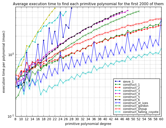
There are some patterns visible in the graph worth noting.
The sieve_1 method is just lousy; for each candidate polynomial we have to compute raising to a power, possibly multiple powers depending on how many factors the period has. Values of \( 2^N-1 \) that are Mersenne primes (\( N=2,3,5,7,13,17,19,31,\ldots \)) don’t have any other prime factors, so they are quicker to verify primitivity, and have lower execution time.
The construct methods other than the St. Ives algorithm all have the same general approach: loop through odd values \( j \) such that \( \gcd(j,2^N-1) = 1 \) and \( j \) is the minimum value in its bitwise rotation. Then use \( j \) to compute the appropriate isomorphism to obtain a new primitive polynomial, whether through LFSR decimation ratios, or minimal polynomials, or characteristic polynomials of powers of a matrix. Most of these algorithms have to do some computations for all odd values of \( j \), not just the values of \( j \) that will yield a primitive polynomial. So the execution time curves tend to have wiggles dependent on the values of \( N \). If \( 2^N-1 \) has lots of factors (like \( N=24, 36, 48 \)) then there is a smaller fraction of primitive polynomials of degree \( N \), and therefore the computation per primitive polynomial is slightly larger.
The construct_1 and construct_2 algorithms use matrices, which have an unfair advantage in that numpy implements them specially in C, so they are faster than a pure Python equivalent. The construct_3 (LFSR decimation) and construct_5 (minimal polynomial calculation, direct) algorithms are very slow. The construct_4 (LFSR decimation, optimized) and construct_6 (minimal polynomial calculation using linear algebra) algorithms are faster. The construct_gordon algorithm is faster but looks to be about the same order of growth as construct_4 and construct_6, and construct_shoup (Shoup’s algorithm) is even faster. But none of these are as fast as the St. Ives algorithm or the Falling Coyote algorithm.
In addition, you may notice a drop in the execution time after \( N=16 \) for some of the construct algorithms, particularly construct_1, construct_2, and construct_falling_coyote. There are 2048 primitive polynomials of degree 16; as N increases beyond this point the number of primitive polynomials increases rapidly, and because we stop after the first 2000 of them, there is a difference of behavior. Why should this matter? Because one of the computational tasks we do, to emit primitive polynomials without repeats, is to discard any value of \( j \) where a bit rotation yields a smaller number. The values of \( j \) which are the minimum of their bitwise rotations, are denser for lower values of \( j \), and in fact if \( j < 2^{\lfloor N/2 \rfloor} \) they are always the minimum of their bitwise rotations. So if we start at low values of \( j \), incrementing by 2 each time, and quit after a threshold that is significantly smaller than the total number of primitive polynomials, we will output a higher fraction of primitive polynomials than for the set of degree-\( N \) polynomials as a whole. This makes it seem as though we need to spend less computational effort per primitive polynomial than for the set of degree-\( N \) polynomials as a whole.
The St. Ives algorithm is unique here, in that we don’t have to do any filtering; every step we take (except when we need to use a new multiplier to traverse the lattice and avoid repeats) yields a new primitive polynomial. The only catch is that the time per polynomial is proportional to the minimum multiplier \( j \) that is relatively prime to \( 2^N-1 \). Odd values of \( N \) can get away with using \( j=3 \), whereas values of \( N \) that are multiples of 12 require at least \( j=11 \), raising the computational time significantly.
Overall the speed champion looks like a close race between the St. Ives and the Falling Coyote algorithms, at least in Python; we would be able to compare more easily over the full range of polynomials by “handicapping” the choice of \( j \) among its bit rotations to a random entry rather than the minimum \( j \), so that the fraction of primitive polynomials is more uniform across the range of possible \( j \) values.
Shoup’s Algorithm may be the fastest for randomly-accessed \( j \); many of the other algorithms rely on updating \( j \) in a deterministic sequence that allows some incremental calculation based on the previous calculation.
If I have time later I will try to implement some of these algorithms (the ones without matrices) in Java and Rust and report back on the results.
Update, September 16, 2018: I have implemented Gordon’s method, Shoup’s algorithm, and the Falling Coyote Algorithm in Java as part of my jlibgf2 library, and have plotted the results below for up to the first 200,000 primitive polynomials per degree. I mentioned above that partial completion is faster because more of the primitive polynomials are found at lower values of \( j \). There is a way to compensate for it, though, by using a different coset representative:
We’ve been using values of \( j \) such that they are the minimum value within their coset, and rejecting any value of \( j \) which has a bit rotation that is less than \( j \).
Instead, we can allow odd values of \( j \) such that \( b(j)=1 \) where
$$ b(j) = \begin{cases}0 & j\, {\rm even},\quad \alpha j \bmod 2^N-1 > 2^i\alpha j \bmod 2^N-1 {\rm\, for\, some\,} i {\rm\, such\, that\,}2^i\cdot j \bmod 2^N-1 {\rm\, is\, odd}\cr 1 & {\rm otherwise}\end{cases}$$
for some value \( \alpha \). Essentially we are rejecting any \( j \) such that \( \alpha j’ \bmod 2^N-1 < \alpha j \bmod 2^N-1 \) for some odd \( j’ \) in the same coset as \( j \). I used the first odd value \( \alpha > \frac{2^N-1}{\phi} \) that is relatively prime to \( 2^N-1 \), with \( \phi = \frac{\sqrt{5}+1}{2} \approx 1.618034. \) The reason this works well is that values of \( j \) which are in the same coset \( J_1 \) will all yield values \( \alpha j \bmod 2^N-1 \) that are in the same coset \( J_2 \) for any \( \alpha \), so it guarantees that exactly one value of \( j \) out of its coset \( J_1 \) will have \( b(j)=1 \), and the multiplication tends to produce pseudorandom values of \( j \) as a coset representative, at least for those values of \( j \) that have several 1 bits in their binary representation.
Here’s an example of this technique for \( N=18 \), showing coset representatives highlighted in green:
N=18
m = (1<<N)-1
phi = (np.sqrt(5)+1)/2
alpha = int(np.floor(m/phi)) | 1
alpha += 10
while gcd(alpha,m) != 1:
    alpha += 2
alpha
162023
i = np.arange(N)
nj = 0
columns = []
columnnames = []
representatives = []
for j0 in xrange(1001,10000,2):
    if gcd(m,j0) != 1:
        continue
    nj += 1
    if nj > 6:
        break
    j = j0
    J1 = []
    J2 = []
    ajmin = m
    reps = []
    for k in xrange(N):
        J1.append(j)
        alphaj = (j*alpha) % m
        if j & 1 and alphaj < ajmin:
            reps = [j,alphaj]
            ajmin = alphaj
        J2.append(alphaj)
        j = (j << 1) % m
    columns += [J1,J2]
    columnnames += ['\\(%d\\)' % j, '\\(%d\\alpha\\)' % j if j > 1 else '\\(\\alpha\\)']
    representatives += reps
columns = np.array(columns).T
df = pd.DataFrame(columns,i,columns=columnnames)
df.index.name = 'i'
representatives = set(representatives)
def highlight(s):
    return ['background-color: #ccffaa' if j in representatives else '' for j in s]
df.style.apply(highlight)| \(1003\) | \(1003\alpha\) | \(1009\) | \(1009\alpha\) | \(1013\) | \(1013\alpha\) | \(1019\) | \(1019\alpha\) | \(1021\) | \(1021\alpha\) | \(1025\) | \(1025\alpha\) | |
|---|---|---|---|---|---|---|---|---|---|---|---|---|
| i | ||||||||||||
| 0 | 1003 | 242552 | 1009 | 166118 | 1013 | 27781 | 1019 | 213490 | 1021 | 13250 | 1025 | 137056 |
| 1 | 2006 | 222961 | 2018 | 70093 | 2026 | 55562 | 2038 | 164837 | 2042 | 26500 | 2050 | 11969 |
| 2 | 4012 | 183779 | 4036 | 140186 | 4052 | 111124 | 4076 | 67531 | 4084 | 53000 | 4100 | 23938 |
| 3 | 8024 | 105415 | 8072 | 18229 | 8104 | 222248 | 8152 | 135062 | 8168 | 106000 | 8200 | 47876 |
| 4 | 16048 | 210830 | 16144 | 36458 | 16208 | 182353 | 16304 | 7981 | 16336 | 212000 | 16400 | 95752 |
| 5 | 32096 | 159517 | 32288 | 72916 | 32416 | 102563 | 32608 | 15962 | 32672 | 161857 | 32800 | 191504 |
| 6 | 64192 | 56891 | 64576 | 145832 | 64832 | 205126 | 65216 | 31924 | 65344 | 61571 | 65600 | 120865 |
| 7 | 128384 | 113782 | 129152 | 29521 | 129664 | 148109 | 130432 | 63848 | 130688 | 123142 | 131200 | 241730 |
| 8 | 256768 | 227564 | 258304 | 59042 | 259328 | 34075 | 260864 | 127696 | 261376 | 246284 | 257 | 221317 |
| 9 | 251393 | 192985 | 254465 | 118084 | 256513 | 68150 | 259585 | 255392 | 260609 | 230425 | 514 | 180491 |
| 10 | 240643 | 123827 | 246787 | 236168 | 250883 | 136300 | 257027 | 248641 | 259075 | 198707 | 1028 | 98839 |
| 11 | 219143 | 247654 | 231431 | 210193 | 239623 | 10457 | 251911 | 235139 | 256007 | 135271 | 2056 | 197678 |
| 12 | 176143 | 233165 | 200719 | 158243 | 217103 | 20914 | 241679 | 208135 | 249871 | 8399 | 4112 | 133213 |
| 13 | 90143 | 204187 | 139295 | 54343 | 172063 | 41828 | 221215 | 154127 | 237599 | 16798 | 8224 | 4283 |
| 14 | 180286 | 146231 | 16447 | 108686 | 81983 | 83656 | 180287 | 46111 | 213055 | 33596 | 16448 | 8566 |
| 15 | 98429 | 30319 | 32894 | 217372 | 163966 | 167312 | 98431 | 92222 | 163967 | 67192 | 32896 | 17132 |
| 16 | 196858 | 60638 | 65788 | 172601 | 65789 | 72481 | 196862 | 184444 | 65791 | 134384 | 65792 | 34264 |
| 17 | 131573 | 121276 | 131576 | 83059 | 131578 | 144962 | 131581 | 106745 | 131582 | 6625 | 131584 | 68528 |
def gcdv(a,b):
    """ vectorized gcd """
    b = np.atleast_1d(b)
    a = a.copy()
    if b.size == 1:
        b = np.ones_like(a)*b
    while np.any(b):
        ai = a[b>0]
        bi = b[b>0]
        qi,ri = divmod(ai, bi)
        a[b>0] = bi
        b[b>0] = ri
    return a

def coset_representatives(N, alpha=1):
    m = (1<<N)-1
    j = np.arange(1,m,2)
    j = j[gcdv(j,m)==1]
    aj = alpha*j % m
    mask = j == j
    ji = j.copy()
    aji = aj.copy()
    for i in xrange(1,N):
        ji = (2*ji) % m
        aji = (2*aji) % m
        j[(ji&1 != 0) & (aj > aji)] = 0
    return j[j>0]

def coset_histogram(N,alpha,ax=None,figsize=None):
    j = coset_representatives(N,alpha)
    if ax is None:
        fig = plt.figure(figsize=figsize)
        ax=fig.add_subplot(1,1,1)
    m = (1<<N)-1
    ax.hist(j,np.linspace(0,m,64))
    ax.set_xlim(0,m)
    ax.set_xlabel('$j$',fontsize=11)
    ax.set_ylabel('bin count',fontsize=11)
    ax.set_title('Histogram of coset representatives for $N=%d, \\alpha=%d$ (%d values of $j$)'
                 % (N,alpha,len(j)), fontsize=11)

fig = plt.figure(figsize=(7,9))
ax = fig.add_subplot(2,1,1)
coset_histogram(18,1,ax=ax)
ax = fig.add_subplot(2,1,2)
coset_histogram(18,alpha,ax=ax)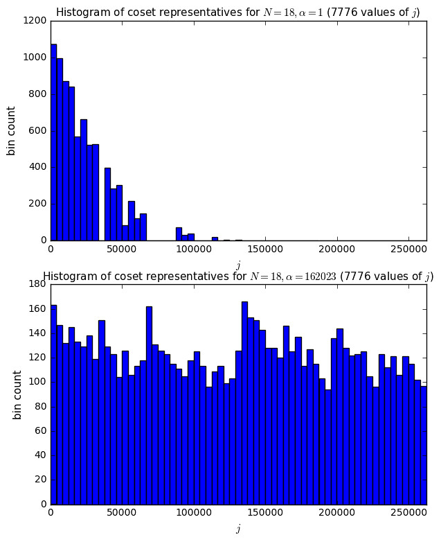
Perhaps not optimal, but the \( \alpha=162063 \) case is much more equally distributed than \( \alpha=1 \), and would better reflect the average time per primitive polynomial if we stop early before finding all primitive polynomials, which is going to be typical for larger values of \( N \).
Anyway here are those timing graphs I mentioned for jlibgf2. The dashed lines are where \( \alpha=1 \); the solid lines are compensated using values of \( \alpha \) described above — except I divide by a power of 2 to keep the resulting \( \alpha < 2^{31} \). There’s a strange drop at \( N=53 \); not sure why that occurs, although it may have to do with the (artificial) constraint I have of keeping \( \alpha < 2^{31} \).
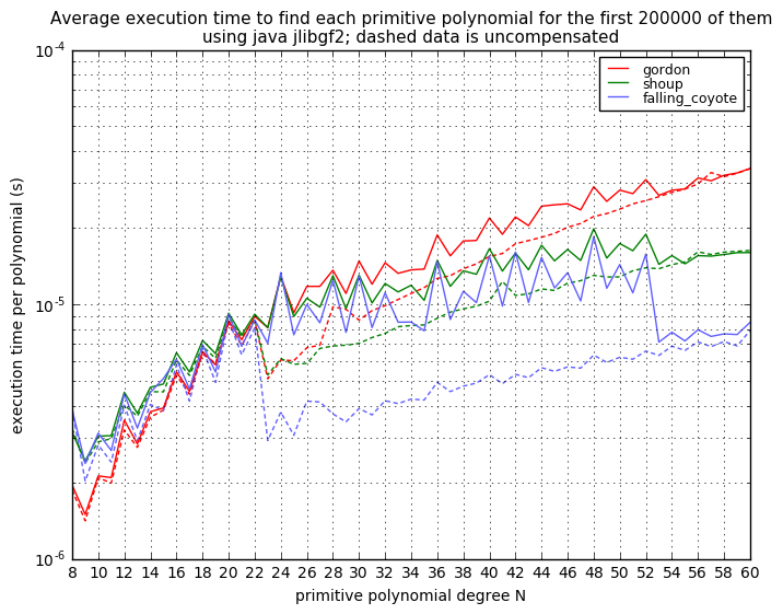
I’ll add the St. Ives algorithm when I have the chance.
Wrapup
We’ve looked at eleven (11!) different techniques for finding primitive polynomials of a given degree \( N \). These boil down to the following general categories:
-
Exhaustive algorithms that take \( O(2^N) \) execution time to verify the minimum period of an LFSR based around the primitive polynomial. These are slow. Don’t bother.
-
Sieve algorithms that use targeted tests to determine whether a given polynomial \( p(x) \) is primitive. The simplest explanation for these is that they determine that \( x^M \bmod p(x) = 1, \) where \( M=2^ N-1 \), and \( x^{(M/q)} \bmod p(x) \ne 1 \) for all prime divisors \( q \mid 2^N-1 \) where \( q < M \). If this is the case, then \( M \) is the smallest positive integer that makes \( x^M \bmod p(x) = 1, \) and \( p(x) \) is a primitive polynomial.
-
Synthetic algorithms or constructive algorithms that can be used to find other primitive polynomials when one primitive polynomial \( p_1(x) \) of the same degree is already known. There are at least two types of these algorithms:
-
Algorithms that find the minimal polynomial \( p_j(x) \) of the element \( x^j \) in the field \( GF(2)[x]/p_1(x) \), where \( \gcd(j,2^N-1) = 1. \) All values \( j \) which are bit rotations share the same minimal polynomial. This approach is equivalent to finding the LFSR with characteristic polynomial \( p_j(x) \) which is decimated by a factor of \( j \) from the LFSR corresponding to \( p_1(x) \): more precisely, it is equivalent to finding with characteristic polynomial \( p_j(x) \) of an LFSR that produces the same output sequence as \( b[jk] \) where \( b[k] \) is the output sequence of the LFSR \( p_1(x) \). (The Berlekamp-Massey algorithm is the usual technique of finding characteristic polynomials of an LFSR that outputs a given sequence.) It is also equivalent to finding the characteristic polynomial of the \( j \)th power of the companion matrix of \( p_1(x) \). These three approaches — minimal polynomial, decimation, and matrix powers — each have their advantages and drawbacks. The Falling Coyote algorithm is a special optimization of the LFSR decimation technique that depends on \( j \) incrementing regularly.
-
Algorithms that find a series of polynomials through repeated decimation by factors \( j \) — the St. Ives algorithm is the only one I’m aware of that can do this.
-
I have measured examples of these algorithms implemented in Python. The St. Ives algorithm and Falling Coyote algorithm seem to be the most efficient of these algorithms.
References
Tables
-
Neal Zierler and John Brillhart, On primitive trinomials (Mod 2), Information and Control, Vol 15, pp. 541-554, 1968.
-
E. J. Watson, Primitive Polynomials (Mod 2), Mathematics of Computation, vol 16 no 79, pp. 368-369, 1962.
-
Miodrag Živković, A Table of Primitive Binary Polynomials, Mathematics of Computation, vol 62 no 205, pp. 385-386, 1994.
Algorithms
-
A. Di Porto, F. Guida and E. Montolivo, Fast algorithm for finding primitive polynomials over GF(q), Electronics Letters, vol 28, no 2, pp. 118-120, January 1992.
-
Nirmal R. Saxena and Edward J. McCluskey, Primitive Polynomial Generation Algorithms: Implementation and Performance Analysis, Center for Reliable Computing Technical Report TR-04-03, Stanford University, April 2004.
-
Sean E. O’Connor, Computing Primitive Polynomials — Theory and Algorithms — O’Connor has given a slightly more rigorous mathematical approach to this topic than other sources I have found.
-
Michael S. Paterson and Larry J. Stockmeyer, On the Number of Nonscalar Multiplications Necessary to Evaluate Polynomials, SIAM Journal on Computing, Vol. 2, No. 1, March 1973.
-
J. A. Gordon, Very simple method to find the minimum polynomial of an arbitrary nonzero element of a finite field, Electronics Letters, vol 12 no 25, December 1976.
-
Victor Shoup, Efficient Computation of Minimal Polynomials in Algebraic Extensions of Finite Fields, ISSAC ‘99 Proceedings of the 1999 international symposium on Symbolic and algebraic computation, July 1999.
-
Eiji Sugimoto, A Short Note on New Indexing Polynomials of Finite Fields, Information and Control vol 41 issue 2, May 1979.
What’s Next?
Next time… well, there will be a next time, but as far as this series goes, this is it. Yes, that’s right — you’ve reached the end! I do plan on providing a short afterword that helps navigate Parts I - XVIII on various topics.
Thanks for reading!
© 2018 Jason M. Sachs, all rights reserved.


- Comments
- Write a Comment Select to add a comment

Hi Jason,
I like your in-depth articles on lfsr's. Its is a lot of information. Maybe you should bundle them into one PDF/book? I would like to have a copy then :-)
Cheers,
Vincent
Hi,
I am in agreement with Vincent. These blog posts are very impressive and I can see them working as a nice book. Where do you get most of your inspiration from?
Ben
To post reply to a comment, click on the 'reply' button attached to each comment. To post a new comment (not a reply to a comment) check out the 'Write a Comment' tab at the top of the comments.
Please login (on the right) if you already have an account on this platform.
Otherwise, please use this form to register (free) an join one of the largest online community for Electrical/Embedded/DSP/FPGA/ML engineers:


