Someday We’ll Find It, The Kelvin Connection

• Circuit Design
• Measurement

You’d think it wouldn’t be too hard to measure electrical resistance accurately. And it’s really not, at least according to wikiHow.com: you just follow these easy steps:

• Choose the item whose resistance you wish to measure.
• Plug the probes into the correct test sockets.
• Turn on the multimeter.
• Select the best testing range.
• Touch the multimeter probes to the item you wish to measure.
• Set the multimeter to a high voltage range after finishing the test.
• Turn off the multimeter.

Somewhere in there, I guess you’re supposed to read the multimeter, but it doesn’t say.

Anyway, for resistances in the 100Ω - 1MΩ range it’s pretty easy. You find a good digital multimeter (DMM), connect probes between it and the two terminals of the resistance in question, and see what the DMM says. Outside this range we have to watch out for parasitic circuit elements causing errors.

Above 1MΩ, things can get a little tricky. If you want better than 1% accuracy for a 1MΩ resistor, that means you need to prevent parasitic parallel resistances from being any lower than 100MΩ. Making high-impedance measurements isn’t an area I’m very familiar with, so I can’t comment on the techniques used. (Except for guard rings, which I never seem to get a chance to use in a design. Oh well.)

Low-impedance measurements, on the other hand, are a source of constant frustration. I deal with resistances under 100Ω all the time. Motor resistances tend to be in the 10mΩ - 10Ω range. At the lower end of this range, even microohms of parasitic series resistance can cause measurement errors.

An ohm is an ohm is an ohm

What is an ohm, anyway? Yeah, we all know it’s an electrical resistance which causes 1 ampere of current to flow when 1 volt is applied across its terminals. But let’s get a sense of how big or small an ohm is.

• Copper wire
  • 14 AWG copper wire, commonly used in house wiring, is 8.286mΩ/m or 82.86 μΩ/cm.
  • 24 AWG copper wire, commonly used for electronics hookup wire, is 84.22mΩ/m or 842.2 μΩ/cm.
  • 28 AWG copper wire, the minimum gauge used in USB cables, is 212.9mΩ/m or 2.129mΩ/cm. That means if you have a cheap 2-meter USB cable that uses 28-gauge wire, and you connect a device that draws 500mA, the voltage drop across each of the power wires is 0.22V, and the 5V at the source port drops down to 4.56V at the device.
  • 30 AWG copper wire, commonly used for PCB rework, is 338.6mΩ/m or 3.386mΩ/cm.
• Copper on printed circuit boards
  • 1oz (35μm) copper, a typical PCB layer thickness, is approximately 0.5 mΩ/square — for a rectangular PCB trace, take the length divided by the width and multiply by the resistance per square. So a 10 mil (0.254mm) width trace that is 2.54mm long has a resistance of 0.5 mΩ × 2.54mm / 0.254mm = 5.0mΩ.
• Solder resistance
  • Solder has typically 11-14% of the electrical conductivity of copper, around 13μΩ·cm.
  • How much resistance does solder add to a through-hole component? We can estimate this. 1/4W through-hole resistors are typically 0.55mm diameter leads; the via holes on a PCB have around 10mil (≈ 0.25mm) diameter clearance, or half of that (5mil ≈ 0.13mm) on the radius. Typical circuit board thickness is 62.5mil = 1.59mm. So a solder connection to the resistor lead has a thickness of 0.13mm and an area of π × 0.6mm × 1.59mm = 3.0mm², and would have a resistance of 13μΩ·cm × 0.13mm / 3.0mm² ≈ 5.6 μΩ. Not very large, but worth noting.
• Connector resistance
  • Analysis of connector contacts is difficult; a concentric pin and socket might only have 3 or 4 small points of contact due to mechanical nonuniformities, with the contact area dependent on the mechanical pressure between the parts. It’s also difficult sometimes to find specifications on contact resistance.
  • Anderson Power Pole PP15-45 connectors: 0.5-0.9mΩ contact resistance (see catalog p. 26)
  • Molex C-Grid connectors: max. 15mΩ contact resistance

Perhaps these give you an idea about resistances of conductors that you usually take for granted.

Practical measurement techniques

So let’s say we’re trying to measure the winding resistance of a motor that we expect to be somewhere around 100mΩ. You could take your multimeter, press the probe tips together, write down the reading (R0), then measure the resistance of the motor winding including the probe resistance (R1), and calculate R1 − R0 as the motor winding resistance. But that’s just asking for trouble. You might have 0.1 - 0.2 Ω series resistance in the probes — which is more than the motor resistance you’re trying to measure, leading to loss of significance — and most DMMs don’t accurately measure resistance that low anyway.

The solution is to use a 4-wire or Kelvin sensing measurement. Some benchtop multimeters have a mode to do this, with four plugs on the front panel, but they tend to be on the expensive side, and it’s just as easy to make a good 4-terminal measurement with a power supply that you can operate in current-limiting mode and a pair of multimeters, one measuring current and one measuring voltage:

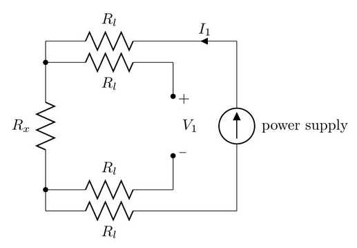
R_x is the unknown resistance, and R_l is the lead resistance. You set the power supply to some current I₁ (something convenient like 1.0A or 5.0A), connect it to R_x through a DMM measuring I₁, and measure the voltage across R_x with another DMM measuring V₁. Then calculate \( R_x = \frac{V_1}{I_1} \).

It’s that easy!

The lead resistances don’t really matter: the outer resistances carry current and have a voltage drop across them, but who cares, because you’re not measuring them in the circuit. The inner resistances don’t carry current so they don’t have any voltage drop across them.

Well, it’s mostly that easy. You still need to be a little careful:

• Worst-case relative error of the measurement is the sum of the relative errors of the two DMMs, at least for small relative errors. If your voltage measurement is ±0.1% accurate and the current measurement is ±0.5% accurate, then your resistance accuracy is ±0.6%. (Don’t believe me? Check it out: \( (V \times 1.001) / (I \times 0.995) = R \times 1.00603 \) and \( (V \times 0.999) / (I \times 1.005) = R \times 0.99403 \). Tada!)

• It’s harder to find DMMs with accurate DC current measurement. I have an Amprobe AM140-A at work. It’s a nice multimeter for the price. You just have to read the fine print. The DC current accuracy at the 5A and 10A ranges is ±0.5% + 20 counts; the accuracy at the 500mA range is ±0.1% + 30 counts. So the best accuracy measurement making a 4-wire measurement with this DMM is to stay just under 500mA. Let’s say we’re at 499.99mA. With this multimeter at the 0.5A peak range, 1 count = 10μA, and 0.1% of 500mA is 500μA, for a net accuracy of 10μA/count × 30 counts + 500μA = 800μA = ± 0.16%. If we have a 2nd DMM of the same type measuring voltage, the voltage reading is more accurate: the manual specifies ±0.03% + 2 counts. We’re measuring a voltage reading of around 50mV so the 2 counts is negligible. Net resistance accuracy would be ± 0.16% for current + ±0.03% for voltage = ± 0.19% for resistance.

• Measuring a really low resistance (< 10mΩ) has the problem of thermoelectric voltages generated across junctions of dissimilar metals, which are typically on the order of a few microvolts. A 10mΩ resistor with 500mA current through it involves a voltage drop of 5mV, and 0.1% accuracy in voltage reading is 5μV, so yeah, a few microvolts matters. The good news is that you can deal with this by making two measurements: first measure the current and voltage, then swap the positive and negative power supply leads and repeat the measurements. Then take the average voltage and the average current of the two measurements, and used these to calculate the resistance. The thermoelectric voltages will cancel out, as well as offsets in the current and voltage measurements of the DMMs.

The four-wire technique is called Kelvin sensing after William Thomson, Lord Kelvin, who invented (among many other achievements) the Kelvin bridge in 1861 as a 4-wire version of the Wheatstone bridge, back in the days before we had accurate analog-to-digital converters. Like balance scales for comparing weights, the idea was that the way to measure resistance was to show equivalence between an unknown resistance and known resistances. Kelvin sensing involves a pair of force/sense connections (or Kelvin connections): the current-carrying path is the “force” connection, and the voltage-measuring path is the “sense” connection.

Resistivity and conductivity measurements

In addition to measuring resistance, 4-wire measurements are used all the time for measuring resistivity (or its inverse, conductivity) of materials. The idea is that if you have a material of known cross-sectional area A and length l, then resistance R, resistivity ρ and conductivity σ are related as follows:

$$ R = \rho\frac{l}{A} = \frac{l}{\sigma A} $$

That’s pretty simple, so you just use a pair of Kelvin connections at the end of a bar of material, right? Well, not quite. The problem with using Kelvin connections to measure conductivity, is that you’d have to use flat plate electrodes at the ends of the material, in order to enforce uniform current density in the material. And it’s a lot easier to use point electrodes. (In fact, if you’re doing fluid conductivity measurements, you can’t use large plate electrodes because they would block the flow of fluid.) So the usual convention is to have a 4-point probe, with all four contacts separated:

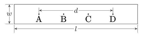
Contacts A and D are the “force” terminals that carry current. They’re placed at some distance d. Contacts B and C are the “sense” terminals that measure current. There is a gap between A and B, and between C and D, so that the current has a chance to spread and curve around, and in the region between B and C the current is uniform.

Here’s an example equipotential plot of the voltage in the right half of the conductor (both halves are symmetric). Let’s assume the voltage at A is 0.000V and the voltage at D is 1.000V. This shows a contour plot of the voltage at any given position in the conductor, and streamlines showing current density:

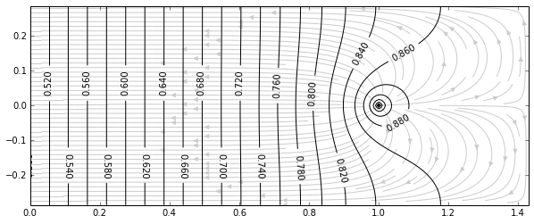
Point (0,0) represents the center, halfway between points A and D. The voltage on the conductor in the vertical line that passes through this point is the average of the voltage applied between A and D, and is labeled showing 0.5. Point (1,0) represents the electrode at point D, which has the label 1.0. Because the electrode is small, the current density is higher near the electrode and a significant voltage drop occurs in the vicinity of the electrode. As you go closer to the center (x=0 on the graph), the voltage variation becomes more uniform.

The conductivity of the material can be calculated as

$$\sigma = \frac{lI}{A_xV}$$

where l is the distance between sense electrodes B and C, A_x is the cross-sectional area of the material, I is the current injected between electrodes A and D, and V is the voltage measured between electrodes B and C. This assumes that the dimensions of the electrodes B and C are small, otherwise they alter the nearby voltage potential.

Material conductivity measurements are kind of a pain, and I’d rather stick with measuring the resistance of a known component.

Kelvin connections in embedded design

There’s another reason to use four-wire measurements. Embedded circuit design is usually voltage-centric: most ADCs measure voltages. If you want to measure currents, you have to route them through a sense resistor and measure the voltage across it. And while finding accurate sense resistors is fairly easy (I’ve already mentioned them as item #9 in an earlier article), you have to be careful with the layout. Here’s an example of a good layout for a current sense resistor:

The wide traces carry current (with an SMT sense resistor spanning the gap). The narrow traces connect directly to the inside edges of the sense resistor’s pads, so that you are measuring the voltages directly across the current sense element. Connect these to a differential amplifier and you’ve got an amplified voltage relative to whatever reference you need. Fairly straightforward, right?

Well, there’s one fly in the ointment.

Remember all those examples I gave at the beginning? They were all examples of the resistance of conductors, which we usually assume is zero, for the sake of convenience. We’re not the only ones to take this resistance for granted. Computer-aided design tools do as well. When you design a circuit in OrCAD or DxDesigner or Altium, the assumption is that you have a series of components connected by ideal conductors. All the component pins that connect to circuit node N14563 are at the same potential.

Except they’re really not, because when current flows along a PCB trace, there is a small but nonzero voltage drop across the trace. And the computer-aided design tools are still in denial about this; or at least, they don’t make it easy.

Quick quiz: how many terminals does the sense resistor (shown above) have? The way you approach circuit layout dictates the answer.

The geometric approach would say that there are two terminals. It’s easy to tell: just count the pads! There are two of them, one below point A and one above point D. Points A and B are the same circuit node (let’s call it SR_PLUS), and points C and D are the same circuit node (let’s call it SR_MINUS). If you want to use a Kelvin connection, you have to diligently make sure the other components on this circuit node are routed properly. Maybe they join the SR_PLUS net at point A. Maybe they join the SR_PLUS net at point B. This information is not included in the schematic, so if you’re the circuit designer and you’re working with your resident PCB layout guy, you have to tell him which traces connect where. Because he doesn’t know all the subtleties of your circuit. And if you’re not careful, he may join the current sense amplifier input to point A, and the MOSFET gate drive chip to point B. Layouts are a multilayer mess that can be difficult to review, so you may not catch all the errors.

The nodal approach would say that there are four terminals. It’s also easy to tell: how many distinct voltages are there? The voltages at point A and B can be different, so they have to be part of different circuit nodes. The same with C and D. So the sense resistor really should have four terminals shown in the schematic, forming four different circuit nodes: perhaps A is called SR_PLUS, B is called SR_PLUS_SENSE, C is called SR_MINUS_SENSE, and D is called SR_MINUS. This makes it really easy to designate in the schematic which components connect to which part of the sense resistor, because that information is captured by the circuit node. You might have a MOSFET with a source pin that connects to SR_PLUS (point A), and a current sense amplifier input that connects to SR_PLUS_SENSE (point B), and there’s no chance of screwing anything up and shorting the two nodes together anywhere except in the sense resistor itself. And here’s the problem with the nodal approach: you do eventually have to join the two Kelvin connections somewhere: SR_PLUS and SR_PLUS_SENSE both need to connect to one terminal of the sense resistor, and SR_MINUS and SR_MINUS_SENSE connect to the other. But the layout tool is designed to prevent inadvertent short circuits, and it knows that it is not allowed to connect two separate circuit nodes together. There is always some clearance distance between the traces of one circuit node and the traces of another. The only way they can interact is through the components. If you want SR_MINUS and SR_MINUS_SENSE to be separate nets in the layout, you can’t connect them with copper in the layout; you have to connect them using an external component, like a jumper. They need to have separate pads. So the sense resistor needs to have four separate pads. Otherwise it will cause errors in the design rule check.

The workaround for the nodal approach is tool-specific, and involves circumventing the usual design rule checks so you can overlap two pads, or connect two nets using a copper pour. I’m not familiar with the “right” way to do this in any of the computer-aided design tools. All I know is that it’s usually a hack.

What you’d really like to have is a component decal that looks sort of like this:

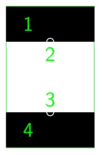
Count the pads: there are 4 of them. Terminals 1 and 4 are the main current-carrying terminals. Terminals 2 and 3 designate a small area along the inside of the current-carrying terminals to be used for Kelvin sensing. Except you just want the little circular gaps between terminals 1 and 2, and between terminals 3 and 4, to be “virtual”, so that the component has 4 virtual terminals but 2 physical pads. As far as I know, though, the PCB design programs don’t have this feature. (Maybe they do now. I don’t know. Drop me a line if you have this feature in your layout tools!)

Somebody thought of that
And someone believed it
And look what it's done so far

In the meantime, be vigilant about your Kelvin connections.

Further reading

• Connector contact resistance
  • A Perspective on Connector Reliability, by Dr. Robert S. Mroczkowski
• Low-resistance measurements
  • Keithley Low Level Measurements Handbook — I found out about this gem about 12 hours after I first posted this article. Keithley has a free downloadable book covering precision DC current, voltage, and resistance measurements, that covers all sorts of useful electrical metrology techniques, and is light on advertising. Yes, of course they have to stop and point out all the Keithley equipment models that can help you with your measurement needs, but what did you expect — a free lunch?
  • Practical Low Resistance Measurements, by Bob Nuckolls
  • The Art of Measuring Low Resistance, by Tee Sheffer and Paul Lantz
  • A Guide to Low Resistance Testing, from Megger Limited
  • Accurate Low-Resistance Measurements Start with Identifying Sources of Error, by Dale Cigoy

© 2014 Jason M. Sachs, all rights reserved.

Sign in