Ten Little Algorithms, Part 5: Quadratic Extremum Interpolation and Chandrupatla's Method

• Applied Math
• Algorithms

Today we will be drifting back into the topic of numerical methods, and look at an algorithm that takes in a series of discretely-sampled data points, and estimates the maximum value of the waveform they were sampled from. This algorithm uses quadratic interpolation, which has applications in the topic of root-finding and minimization. As a bonus, we’ll also look at a nifty root-finding method that uses quadratic interpolation as well.

You’ve probably heard of linear interpolation, where you are trying to find a point along the line containing the points \( (x_1, y_1) \) and \( (x_2, y_2) \). There’s not much to say about it; if you have an x-coordinate \( x \) then the corresponding y-coordinate is \( y = y_1 + \frac{y_2-y_1}{x_2-x_1}(x-x_1) \). The inversion of the problem looks the same: given a y-coordinate \( y \), find the x-coordinate by computing \( x = x_1 + \frac{x_2-x_1}{y_2-y_1}(y-y_1) \). Both are linear in \( x \) and \( y \).

What if we had three points \( p_1 = (x_1, y_1) \), \( p_2 = (x_2, y_2) \), and \( p_3 = (x_3, y_3) \) and we wanted to find a curve with a quadratic equation that passes through all three of them?

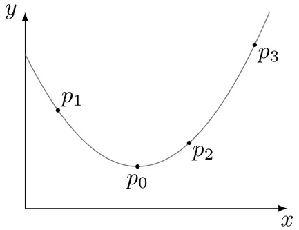
This is an example of Lagrange interpolation, and the form of the equation is roughly the same as linear interpolation, only with more stuff:

$$ y = y_1 \left(\frac{x-x_2}{x_1-x_2}\cdot\frac{x-x_3}{x_1-x_3}\right) + y_2 \left(\frac{x-x_1}{x_2-x_1}\cdot\frac{x-x_3}{x_2-x_3}\right) + y_3 \left(\frac{x-x_1}{x_3-x_1}\cdot\frac{x-x_2}{x_3-x_2}\right) $$

When you evaluate it at one of the three points, each of the parenthesized fractions here has a value of 1 or 0; the first term, for example, has a value of zero if \( x = x_2 \) or \( x = x_3 \), and a value of \( y_1 \) if \( x = x_1 \).

Rather than getting stuck in another game of Grungy Algebra again, let’s use an example:

• \( p_1 = (1,3) \)
• \( p_2 = (5,2) \)
• \( p_3 = (7,5) \)

If we run through Lagrange’s formula, we get

$$\begin{eqnarray} y &=& 3 \frac{x-5}{1-5}\cdot\frac{x-7}{1-7} + 2\frac{x-1}{5-1}\cdot\frac{x-7}{5-7} + 5\frac{x-1}{7-1}\cdot\frac{x-5}{7-5} \cr &=& \tfrac{3}{24}(x^2 - 12x + 35) - \tfrac{6}{24}(x^2 - 8x + 7) + \tfrac{10}{24}(x^2 - 6x + 5) \cr &=& \tfrac{1}{24}(7x^2 - 48x + 113) \end{eqnarray}$$

Now that we have this equation, we could find the minimum of the parabola; for a quadratic equation \( ax^2 + bx + c \), the minimum occurs at \( x = -\frac{b}{2a} \), so if we plug in \( x = \frac{24}{7} \) and do all the arithmetic, we get \( y = \frac{215}{168} \), so the point shown is \( p_0 = (\frac{24}{7}, \frac{215}{168}) \).

OK, great — so what?

Finding a maximum between samples

Let’s say we have some regularly-sampled data and we want to find the maximum value of a waveform. Here’s the step response of a second-order system with natural frequency 405 rad/s and damping factor \( \zeta=0.52 \):

import numpy as np
import matplotlib.pyplot as plt
import scipy.signal

# step response of 1/(s^2/w0^2 + 2*zeta*s/w0 + 1)
w0 = 405
zeta = 0.52
H = scipy.signal.lti([1],[1.0/w0/w0, 2*zeta/w0, 1])
t,y=scipy.signal.step(H,T=np.arange(0,0.01401,0.0002))
plt.plot(t,y)
t1,y1=scipy.signal.step(H,T=np.arange(0,0.01401,0.002))
plt.plot(t1,y1,'.')
for tj,yj in zip(t1[4:7],y1[4:7]):
    plt.text(tj,yj,'\n%.5f'%yj,verticalalignment='top')

If we wanted to find the maximum value of this waveform, we could try to find a closed-form equation and then find its maximum. But that’s not an easy problem in general; it can be done in limited cases (like step responses) but not for the response of general input waveforms.

Alternatively, we could try to get the maximum value numerically. We will get a more accurate answer the closer these sampling points are. But that comes with a cost. We’d have to simulate more samples, and our simulation might be expensive.

One approach we could use is to find the maximum value of the sampled points, and look at its two adjacent neighbors, and then fit a parabola to these points. Here we have \( t_0 = 0.008 \), \( t_1 = 0.010 \), and \( t_2 = 0.012 \).

This is a much easier interpolation effort. We can rescale the x-axis as \( u - \frac{t-t_1}{\Delta t} \) with \( \Delta t \) = the sampling interval; then this equation becomes

$$ \begin{eqnarray} y _ 0 &=& \left.au^2 + bu + c\right| _ {u=-1} &= a-b+c \cr y _ 1 &=& \left.au^2 + bu + c\right| _ {u=0} &= c\cr y _ 2 &=& \left.au^2 + bu + c\right| _ {u=1} &= a+b+c \end{eqnarray} $$

and then we have \( c = y_1 \), \( b = \frac{1}{2}(y_2 - y_0) \), and \( a = \frac{1}{2}(y_2 + y_0) - c \). With our example system, that means \( c = 1.13878 \), \( b = -0.023854 \), and \( a = -0.031247 \).

The maximum value of this polynomial occurs at \( u=-\frac{b}{2a} \). This is true for all quadratic equations (remember completing the square from high school math?). At this value of \( u \), \( y = a\frac{b^2}{4a^2} - b\frac{b}{2a} + c = c - \frac{b^2}{4a} \).

plt.plot(t,y,'b')
plt.xlim(0.0079, 0.0121)
plt.ylim(1.05,1.2)
tpts = t1[4:7]
ypts = y1[4:7]
plt.plot(tpts,ypts,'b.',markersize=8)

c = ypts[1]
b = (ypts[2]-ypts[0])/2.0
a = (ypts[2]+ypts[0])/2.0 - c
print a,b,c
t2 = np.arange(0.008,0.012,0.0001)
u2 = (t2 - tpts[1])/(tpts[1]-tpts[0])
plt.plot(t2,a*u2*u2 + b*u2 + c,'r--')
t3 = (tpts[1]-tpts[0])*(-b/2.0/a) + tpts[1]
y3 = c - b*b/4.0/a
plt.plot(t3,y3,'r.', markersize=8)
plt.annotate('(%.5f,%.5f)' % (t3,y3), xy=(t3,y3),
             xytext = (0.009,1.12), horizontalalignment='center',
             arrowprops = dict(arrowstyle="->"))

-0.0312470769869 -0.0238536034466 1.13878353174

We predict an overshoot of 0.14334. The actual overshoot here is \( e^{-\pi \frac{\zeta}{\sqrt{1-\zeta^2}}} \); for \( \zeta=0.52 \) we get 0.14770 instead. Not bad. Here’s the whole algorithm:

def qinterp_max(y, extras=False):
    '''
    Find the maximum point in an array, and if it's an interior point,
    interpolate among it and its two nearest neighbors to predict
    the interpolated maximum.
    
    Returns that interpolated maximum,
    if extras=True, also returns the coefficients
    and the index and value of the sample maximum.
    '''
    imax = 0
    ymax = -float('inf')
    # run through the points to find the maximum
    for i,y_i in enumerate(y):
        if y_i > ymax:
            imax = i
            ymax = y_i
    # no interpolation if at the ends
    if imax == 0 or imax == i-1:
        return ymax
    # otherwise, y[imax] >= either of its neighbors,
    # and we use quadratic interpolation:
    c = y[imax]
    b = (y[imax+1]-y[imax-1])/2.0
    a = (y[imax+1]+y[imax-1])/2.0 - c
    yinterp = c - b*b/4.0/a
    if extras:
        return yinterp, (a,b,c), imax, ymax
    else:
        return yinterp

OK, now let’s use it and see how its accuracy varies with step size:

ymax_actual = 1+np.exp(-np.pi*zeta/np.sqrt(1-zeta**2))
print 'actual peak: ', ymax_actual

def fit_power(x,y):
    lnx = np.log(x)
    lny = np.log(np.abs(y))
    A = np.vstack((np.ones(lnx.shape), lnx)).T
    c,m = np.linalg.lstsq(A, lny)[0]
    C = np.exp(c)
    return C,m

dt_array = []
errq_array = []
err_array = []
for k in xrange(10):
    delta_t = 0.002 / (2**k)
    dt_array.append(delta_t)
    t,y=scipy.signal.step(H,T=np.arange(0,0.015,delta_t))
    ymax_interp, coeffs, imax, ymax = qinterp_max(y, extras=True)
    err = ymax - ymax_actual
    err_array.append(err)
    errq = ymax_interp - ymax_actual
    errq_array.append(errq)
    print '%d %.6f %.8f %g' % (k, delta_t, ymax_interp, errq)
C,m = fit_power(dt_array, err_array)
print 'sampled error ~= C * dt^m; C=%f, m=%f' % (C,m)
C,m = fit_power(dt_array, errq_array)
print 'interpolated error ~= C * dt^m; C=%f, m=%f' % (C,m)
plt.loglog(dt_array, np.abs(err_array), '+', dt_array, np.abs(errq_array),'.')
dt_bestfit = [2e-6, 5e-3]
plt.plot(dt_bestfit,C*dt_bestfit**m,'--')
plt.grid('on')
plt.xlabel('$\Delta t$', fontsize=15)
plt.ylabel('error')
plt.legend(('sampled','interpolated'), loc='best')

actual peak:  1.14770455973
0 0.002000 1.14333591 -0.00436865
1 0.001000 1.14789591 0.000191353
2 0.000500 1.14774129 3.67308e-05
3 0.000250 1.14771241 7.84859e-06
4 0.000125 1.14770355 -1.01057e-06
5 0.000063 1.14770467 1.14566e-07
6 0.000031 1.14770454 -1.72937e-08
7 0.000016 1.14770456 1.30011e-09
8 0.000008 1.14770456 2.79934e-10
9 0.000004 1.14770456 -1.62288e-11
sampled error ~= C * dt^m; C=382.019171, m=1.923258
interpolated error ~= C * dt^m; C=326991.894388, m=2.977363

Our interpolated error has a very clear cubic dependency on the timestep Δt. This makes sense: pretty much whenever you are using a polynomial method of degree \( n \), you will get an error that is a polynomial of degree \( n+1 \). So if I divide the timestep by 10, my error will decrease by a factor of around 1000.

The uninterpolated error has a quadratic dependency on the timestep Δt. So quadratic interpolation in this case is a clear winner for small timesteps. What constitutes a small timestep? Well, in order for interpolation to be accurate, the data needs to be smooth, and “quadratic-looking”. Perhaps if you use Chebyshev approximation to fit a quadratic to a series of 5-10 successive points, and you compare the residuals to the magnitude of the Chebyshev quadratic component, you’d get an idea. Let’s just try that for two timesteps. Looking at the graph, it seems like a timestep of 10^-3 is not very quadratic (interpolation actually gives us a slightly higher error than taking the raw samples), but a timestep of 10^-4 is reasonably quadratic.

for delta_t in [1e-3, 1e-4]:
    t,y=scipy.signal.step(H,T=np.arange(0,0.015,delta_t))
    ymax_interp, coeffs, imax, ymax = qinterp_max(y, extras=True)
    tt = t[imax-5:imax+6]
    yy = y[imax-5:imax+6]
    fig = plt.figure()
    ax = fig.add_subplot(1,1,1)
    ax.plot(tt,yy, '.')
    
    a,b,c = coeffs
    tinterp = np.linspace(tt[0],tt[-1],100)
    uinterp = (tinterp - t[imax])/delta_t
    plt.plot(tinterp, a*uinterp**2 + b*uinterp + c, '--')
    plt.plot(t[imax] - b/2.0/a *delta_t, ymax_interp, 'x')
    plt.legend(('sample points','quadratic eqn containing\nmax + 2 neighbors','quad interpolated max'), loc='best')
    
    # find u linearly related to tt such that u spans the interval -1 to +1
    u = (tt*2 - (tt[-1] + tt[0])) / (tt[-1] - tt[0])
    coeffs, extra = np.polynomial.chebyshev.chebfit(u,yy,2,full=True)
    rms_residuals = np.sqrt(extra[0][0])
    print 'coeffs=',coeffs, 'RMS residual=',rms_residuals

coeffs= [ 0.99384519  0.13676706 -0.15229459] RMS residual= 0.10100632695
coeffs= [  1.14619769e+00  -7.34868794e-05  -1.50279049e-03] RMS residual= 0.000133276857498

In the first case, with timestep = 10^-3, the RMS of the residuals is almost as large as the magnitude of the quadratic component; with timestep = 10^-4, the RMS of the residuals is only about a tenth as large as the magnitude of the quadratic component.

Yes, we could use more points and/or fit a cubic or a quartic equation to them, but quadratic interpolation based on three sample points is fast and simple, and does the job.

Root-finding and Chandrupatla’s Method

Today you’re going to get two algorithms for the price of one. This article was originally going to be about Brent’s method for finding the root of an equation numerically. It is an improvement developed by Richard Brent in 1973, on an earlier algorithm developed by T.J. Dekker in 1969. Brent’s method is awesome! It’s the de facto standard for root-finding of a single-variable function, used in scipy.optimize.brentq in Python, org.apache.commons.math3.analysis.solvers.BrentSolver in Java, and fzero in MATLAB.

Let’s say you want to find some value of x such that \( \tan x - x = 0.1 \). This is a nonlinear equation with a non-algebraic solution: we’re not going to find a closed-form solution in terms of elementary functions. All we have to do is define a function \( f(x) = \tan x - x - 0.1 \) and bound some interval such that the function is continuous within that interval, and when \( f(x) \) is evaluated at the endpoints of that interval, they have opposite signs. This is called bracketing the root. That’s pretty easy: \( f(0) = -0.1 \) and \( f(\pi/4) = 0.9 - \pi/4 \approx 0.115 \).

Then we run Brent’s method with the input of \( f(x) \) and the interval \( x \in [0, \pi/4] \):

import scipy.optimize

def f(x):
    return np.tan(x) - x - 0.1

x1 = scipy.optimize.brentq(f, 0, np.pi/4)
print 'x=',x1, 'f(x1)=',f(x1)

x = np.arange(0, 0.78, 0.001)
plt.plot(x, np.tan(x) - x)
plt.plot(x1, np.tan(x1) - x1, '.', markersize=8)
plt.grid('on')

x= 0.631659472661 f(x1)= 1.94289029309e-16

There’s only one problem: Brent’s method is… um… well I’d call it unsatisfying. It works very well by alternating between three different kinds of iteration steps to narrow the bracket around the root, but it’s very heuristic in doing this.

General root-finding methods are very tricky, because functions themselves can be full of crazy nasty behaviors. (Just look at the Weierstrass function.) I’m not going to cover the whole topic of root-finding: it’s long and full of pitfalls, and you want to use a library function when you can. So here’s the 3-minute version, applicable to continuous functions of one variable within a given interval bracketing a root:

• The simple robust algorithm is bisection, where we evaluate the function at the interval midpoint, guaranteeing that one of the half-intervals also brackets a root. This converges linearly, taking roughly 53 steps for 64-bit IEEE-754 double-precision calculations since they contain a 53-bit mantissa, and bisection gains one bit of precision at each iteration.

• The faster algorithms include things like Newton’s method, the secant method, and inverse quadratic interpolation, which converge much more quickly… except sometimes they don’t converge at all. Newton’s method requires either a closed-form expression for a function’s derivative, or extra evaluations to calculate that derivative; the secant method is similar but doesn’t require derivatives. These methods take advantage of the fact that most functions become smoother when you narrow the interval of evaluation, so they look more linear, and the higher-degree components of their polynomial approximation become smaller.

Brent’s method switches back and forth between these methods based on some rules he proved would guarantee worst-case convergence.

While looking for a good explanation of Brent’s method, I stumbled across a reference to a newer algorithm developed by Tirupathi Chandrupatla in 1997. Chandrupatla is a professor of mechanical engineering at Rowan University in southern New Jersey; this algorithm appears to be mentioned only in his original article published in 1997 in an academic journal, and described second-hand in a book on computational physics by Philipp Scherer. Scherer’s description is very usable, and includes comparisons between Chandrupatla’s method and several other root-finding methods including Brent’s method, but it doesn’t give much background on why Chandrupatla’s method works. I haven’t been able to access Chandrupatla’s original article, but the description in Scherer’s book is easy enough to implement in Python and compare to other methods.

Chandrupatla’s method is both simpler than Brent’s method, and converges faster for functions that are flat around their roots (which means they have multiple roots or closely-located roots). Basically it uses either bisection or inverse quadratic interpolation, based on a relatively simple criteria. Inverse quadratic interpolation is just quadratic interpolation using the y-values as inputs and the x-value as output.

Here’s an example of inverse quadratic interpolation. Let’s say we have our function \( f(x) = \tan x - x - 0.1 \) and we have three points \( (x_1, y_1) \), \( (x_2, y_2) \), and \( (x_3, y_3) \), with \( x_1 = 0.5, x_2 = 0.65, x_3 = 0.8 \). We use Lagrange’s quadratic interpolation formula mentioned earlier, but swapping the x and y values:

$$ x = x_1 \left(\frac{y-y_2}{y_1-y_2}\cdot\frac{y-y_3}{y_1-y_3}\right) + x_2 \left(\frac{y-y_1}{y_2-y_1}\cdot\frac{y-y_3}{y_2-y_3}\right) + x_3 \left(\frac{y-y_1}{y_3-y_1}\cdot\frac{y-y_2}{y_3-y_2}\right) $$

And we just plug in \( y=0 \) to find an estimate of the corresponding value for x:

def iqi(f, x1, x2, x3):
    y1 = f(x1)
    y2 = f(x2)
    y3 = f(x3)
    def g(y):
        return (x1*(y-y2)*(y-y3)/(y1-y2)/(y1-y3)
              + x2*(y-y1)*(y-y3)/(y2-y1)/(y2-y3)
              + x3*(y-y1)*(y-y2)/(y3-y1)/(y3-y2))
    return g

def f(x):
    return np.tan(x) - x - 0.1

g = iqi(f, 0.5, 0.65, 0.8)
x3 = g(0)
print 'x3=',x3, 'f(x3)=',f(x3)

x = np.arange(0.5,0.8,0.001)
y = f(x)
plt.plot(x,y,'-',g(y),y,'--')
plt.plot([0.5, 0.65, 0.8],f(np.array([0.5,0.65,0.8])),'.',markersize=8)
plt.xlim(0.5,0.8)
plt.grid('on')
plt.plot(x3,f(x3),'g+',markersize=8)
plt.legend(('f(x)','inv quad interp'),loc='best')

x3= 0.629308756053 f(x3)= -0.00125220861941

We get a much more accurate estimate. (The reason we use inverse quadratic interpolation rather than quadratic interpolation is that the latter requires solving a quadratic equation numerically, which requires a square root operation.) It works very well for smooth functions that are mostly linear and a little bit quadratic. But sometimes it fails and bisection is a reliable backup. So here’s Chandrupatla’s algorithm; I’ve added a few comments to help explain some of it.

def chandrupatla(f,x0,x1,verbose=False, eps_m = None, eps_a = None):
    # adapted from Chandrupatla's algorithm as described in Scherer
    # https://books.google.com/books?id=cC-8BAAAQBAJ&pg=PA95
    
    # Initialization
    b = x0
    a = x1
    c = x1
    fa = f(a)
    fb = f(b)
    fc = fa
    # Make sure we are bracketing a root
    assert np.sign(fa) * np.sign(fb) <= 0    
    t = 0.5
    do_iqi = False
    
    # jms: some guesses for default values of the eps_m and eps_a settings
    # based on machine precision... not sure exactly what to do here
    eps = np.finfo(float).eps
    if eps_m is None:
        eps_m = eps
    if eps_a is None:
        eps_a = 2*eps
    
    while True:
        # use t to linearly interpolate between a and b,
        # and evaluate this function as our newest estimate xt
        xt = a + t*(b-a)
        ft = f(xt)
        if verbose:
            print  '%s t=%f xt=%f ft=%g a=%f b=%f c=%f' % (
               'IQI' if do_iqi else 'BIS', t, xt, ft, a, b, c) 
        # update our history of the last few points so that
        # - a is the newest estimate (we're going to update it from xt)
        # - c and b get the preceding two estimates
        # - a and b maintain opposite signs for f(a) and f(b)
        if np.sign(ft) == np.sign(fa):
            c = a
            fc = fa
        else:
            c = b
            b = a
            fc = fb
            fb = fa
        a = xt
        fa = ft
        # set xm so that f(xm) is the minimum magnitude of f(a) and f(b)
        if np.abs(fa) < np.abs(fb):
            xm = a
            fm = fa
        else:
            xm = b
            fm = fb
        if fm == 0:
            return xm
        # Figure out values xi and phi 
        # to determine which method we should use next
        tol = 2*eps_m*np.abs(xm) + eps_a
        tlim = tol/np.abs(b-c)
        if tlim > 0.5:
            return xm
        
        xi  = (a-b)/(c-b)
        phi = (fa-fb)/(fc-fb)
        do_iqi = phi**2 < xi and (1-phi)**2 < 1-xi
            
        if do_iqi:
            # inverse quadratic interpolation
            t = fa / (fb-fa) * fc / (fb-fc) + (c-a)/(b-a)*fa/(fc-fa)*fb/(fc-fb)
        else:
            # bisection
            t = 0.5
        
        # limit to the range (tlim, 1-tlim)
        t = np.minimum(1-tlim, np.maximum(tlim, t))

Let’s give it a spin to find \( \sqrt{2} \):

def tracker(f, a=0):
    ''' decorates calls to f(x) to track each call '''
    i = [0]
    def g(x):
        i[0] += 1
        y = f(x)
        print "i=%2d, x=%f, y=%f, err=%g" % (i[0],x,y,y-a)
        return y-a
    return g
    
chandrupatla(tracker(lambda x: x**2, 2),1,2,verbose=True)

i= 1, x=2.000000, y=4.000000, err=2
i= 2, x=1.000000, y=1.000000, err=-1
i= 3, x=1.500000, y=2.250000, err=0.25
BIS t=0.500000 xt=1.500000 ft=0.25 a=2.000000 b=1.000000 c=2.000000
i= 4, x=1.409524, y=1.986757, err=-0.0132426
IQI t=0.180952 xt=1.409524 ft=-0.0132426 a=1.500000 b=1.000000 c=2.000000
i= 5, x=1.414264, y=2.000143, err=0.000143176
IQI t=0.052394 xt=1.414264 ft=0.000143176 a=1.409524 b=1.500000 c=1.000000
i= 6, x=1.414214, y=2.000000, err=-1.38041e-08
IQI t=0.010679 xt=1.414214 ft=-1.38041e-08 a=1.414264 b=1.409524 c=1.500000
i= 7, x=1.414214, y=2.000000, err=8.88178e-16
IQI t=0.000096 xt=1.414214 ft=8.88178e-16 a=1.414214 b=1.414264 c=1.409524
i= 8, x=1.414214, y=2.000000, err=4.44089e-16
IQI t=0.000000 xt=1.414214 ft=4.44089e-16 a=1.414214 b=1.414214 c=1.414264
i= 9, x=1.414214, y=2.000000, err=-2.88658e-15
IQI t=0.000000 xt=1.414214 ft=-2.88658e-15 a=1.414214 b=1.414214 c=1.414214
i=10, x=1.414214, y=2.000000, err=-4.44089e-16
IQI t=0.866667 xt=1.414214 ft=-4.44089e-16 a=1.414214 b=1.414214 c=1.414214

It worked! The first iteration was handled by bisection, but after that we ended up using inverse quadratic interpolation to converge quickly. It looks like I gave it poor termination criteria for the eps_m and eps_a numbers; it gets to nearly machine precision at iteration 7, and then mumbles around before giving up. And here’s Brent’s method:

scipy.optimize.brentq(tracker(lambda x: x**2, 2),1,2)

i= 1, x=1.000000, y=1.000000, err=-1
i= 2, x=2.000000, y=4.000000, err=2
i= 3, x=1.333333, y=1.777778, err=-0.222222
i= 4, x=1.419048, y=2.013696, err=0.0136961
i= 5, x=1.414072, y=1.999598, err=-0.000401762
i= 6, x=1.414213, y=1.999999, err=-6.85547e-07
i= 7, x=1.414214, y=2.000000, err=1.1724e-13
i= 8, x=1.414214, y=2.000000, err=-2.71294e-12

Let’s look at a function that’s nasty to solve because of its flatness, and requires bisection for a couple of terms:

chandrupatla(tracker(lambda x: np.cos(x) - 0.999),-0.01,0.8,verbose=True)

i= 1, x=0.800000, y=-0.302293, err=-0.302293
i= 2, x=-0.010000, y=0.000950, err=0.00095
i= 3, x=0.395000, y=-0.076003, err=-0.0760034
BIS t=0.500000 xt=0.395000 ft=-0.0760034 a=0.800000 b=-0.010000 c=0.800000
i= 4, x=0.192500, y=-0.017471, err=-0.017471
BIS t=0.500000 xt=0.192500 ft=-0.017471 a=0.395000 b=-0.010000 c=0.800000
i= 5, x=0.091250, y=-0.003160, err=-0.00316039
BIS t=0.500000 xt=0.091250 ft=-0.00316039 a=0.192500 b=-0.010000 c=0.395000
i= 6, x=0.040625, y=0.000175, err=0.000174918
BIS t=0.500000 xt=0.040625 ft=0.000174918 a=0.091250 b=-0.010000 c=0.192500
i= 7, x=0.065937, y=-0.001173, err=-0.00117309
BIS t=0.500000 xt=0.065937 ft=-0.00117309 a=0.040625 b=0.091250 c=-0.010000
i= 8, x=0.044281, y=0.000020, err=1.97482e-05
IQI t=0.855558 xt=0.044281 ft=1.97482e-05 a=0.065937 b=0.040625 c=0.091250
i= 9, x=0.044733, y=-0.000000, err=-3.38295e-07
IQI t=0.020847 xt=0.044733 ft=-3.38295e-07 a=0.044281 b=0.065937 c=0.040625
i=10, x=0.044725, y=0.000000, err=5.85319e-10
IQI t=0.016787 xt=0.044725 ft=5.85319e-10 a=0.044733 b=0.044281 c=0.065937
i=11, x=0.044725, y=-0.000000, err=-4.44089e-16
IQI t=0.001727 xt=0.044725 ft=-4.44089e-16 a=0.044725 b=0.044733 c=0.044281
i=12, x=0.044725, y=0.000000, err=0
IQI t=0.000001 xt=0.044725 ft=0 a=0.044725 b=0.044725 c=0.044733

scipy.optimize.brentq(tracker(lambda x: np.cos(x) - 0.999),-0.01,0.8)

i= 1, x=-0.010000, y=0.000950, err=0.00095
i= 2, x=0.800000, y=-0.302293, err=-0.302293
i= 3, x=-0.007462, y=0.000972, err=0.000972156
i= 4, x=0.396269, y=-0.076492, err=-0.0764924
i= 5, x=-0.002396, y=0.000997, err=0.00099713
i= 6, x=0.196937, y=-0.018329, err=-0.0183294
i= 7, x=0.007889, y=0.000969, err=0.000968885
i= 8, x=0.102413, y=-0.004240, err=-0.00423958
i= 9, x=0.025472, y=0.000676, err=0.000675605
i=10, x=0.060410, y=-0.000824, err=-0.000824129
i=11, x=0.041211, y=0.000151, err=0.000150947
i=12, x=0.045038, y=-0.000014, err=-1.40481e-05
i=13, x=0.044712, y=0.000001, err=5.69923e-07
i=14, x=0.044725, y=0.000000, err=1.98721e-09
i=15, x=0.044725, y=-0.000000, err=-1.9984e-15
i=16, x=0.044725, y=0.000000, err=4.27436e-14

We can even write a function to investigate the rate of convergence using graphs like those given in Scherer’s book:

def show_converge_brent_chandrupatla(f, a, b, title=None):
    def track_history(f):
        xh = []
        def g(x):
            xh.append(x)
            return f(x)
        return g, xh
    fbrent, xbrent = track_history(f)
    fchand, xchand = track_history(f)
    scipy.optimize.brentq(fbrent, a, b)
    chandrupatla(fchand, a, b)
    xbrent = np.array(xbrent)
    xchand = np.array(xchand)
    fig = plt.figure()
    ax = fig.add_subplot(1,1,1)
    for x,s in ((xbrent,'.'),(xchand,'+')):
        ax.semilogy(np.arange(len(x)), np.abs(f(x)), s)
    ax.legend(('Brent','Chandrupatla'), loc='best')
    ax.set_xlabel('iteration')
    ax.set_ylabel('error')
    if title is not None:
        fig.suptitle(title, fontsize=18)
        
show_converge_brent_chandrupatla(lambda x: x*x-2, 0, 2, '$x^2-2$')
show_converge_brent_chandrupatla(lambda x: np.cos(x)-0.999, -0.01, 0.8, '$\\cos\ x - 0.999$')
show_converge_brent_chandrupatla(lambda x: (x-1.7)**17, 0, 2, '$(x-1.7)^{17}$')
        

Chandrupatla’s method is either comparable to Brent’s method, or (in the case of multiple roots or local flatness) converges faster.

In fact, I would have focused this article completely on Chandrupatla’s algorithm… except that I don’t understand the part about \( \xi \) and \( \Phi \) which picks whether bisection or inverse quadratic interpolation is used. Boo. Not completely satisfying.

So you get my maximum-interpolation algorithm instead.

Summary

Today we looked at two algorithms that use Lagrange’s formula for interpolating a quadratic polynomial to three given points:

• an algorithm that uses quadratic interpolation to give a better estimate of the maximum of regularly-sampled data (for good results, the data must be smooth and have enough samples so that near the maximum, it has low content of degree 3 or higher — do not use digitized samples from an ADC for this!)

• Chandrupatla’s method, a relatively new algorithm for finding roots of functions of one variable. It is underdocumented and underappreciated, and appears to be simpler than Brent’s method, with equal or better rate of convergence.

For more information on root finding algorithms, here are some references:

• Numerical Recipes, by Press, Teukolsky, Vetterling and Flannery. You should have one of these books (pick your favorite implementation language) on your bookshelf. The algorithm descriptions are great. The code is very difficult to read, using lots of one- or two-letter variable names with cryptic Fortran-style designs, but it’s a start.

• Cleve Moler’s Cleve’s Corner series on the “Zeroin” algorithm designed by T. J. Dekker, improved by Brent, and incorporated into MATLAB’s fzero

• Richard Brent’s posting of the old out-of-print edition of his book Algorithms for Minimization Without Derivatives in PDF format. Brent’s method for finding roots starts on p. 47. Warning: this is a rigorous math text, so it has lots of theory, and it’s old enough that the sample algorithm is implemented in ALGOL 60.

© 2015 Jason M. Sachs, all rights reserved.

Sign in