


Ten Little Algorithms, Part 6: Green’s Theorem and Swept-Area Detection
Other articles in this series:
- Part 1: Russian Peasant Multiplication
- Part 2: The Single-Pole Low-Pass Filter
- Part 3: Welford's Method (And Friends)
- Part 4: Topological Sort
- Part 5: Quadratic Extremum Interpolation and Chandrupatla's Method
This article is mainly an excuse to scribble down some cryptic-looking mathematics — Don’t panic! Close your eyes and scroll down if you feel nauseous — and share a very simple and useful signal processing algorithm for detecting real-time rotation in a plane.
$$ \oint_C P\,dx + Q\, dy = \int\!\!\!\int_R \left({\partial Q\over \partial x} - {\partial P\over \partial y}\right) \,dA $$
That’s Green’s Theorem, which says that you can relate the line integral around a plane curve \( C \) with a double-integral over the area \( R \) contained within \( C \).
$$ \oint_C \mathbf{F} \cdot d\mathbf{r} = \int\!\!\!\int_S \left(\nabla \times \mathbf{F}\right) \cdot d\mathbf{S} $$
That’s Stokes’s Theorem (actually the Kelvin-Stokes Theorem), which is a generalization of Green’s Theorem to three dimensions, and says that the line integral around a curve \( C \) in three-dimensional space is equal to an area integral over a surface \( S \) that has \( C \) as a boundary.
There’s also the Divergence Theorem which is related, but I’ve used up my allocation of cryptic-looking mathematics already, so just forget I mentioned it.
If you want some insight into this kind of stuff (which is NOT the point of this article) here are a couple of good references:
- Green’s Theorem on the Khan Academy website
- David Halliday and Robert Resnick’s Fundamentals of Physics (aka “Halliday and Resnick”), which is one of the classic physics textbooks, and talks about electromagnetics and vector fields; this stuff becomes useful when you start getting into Maxwell’s equations.
- H.M. Schey’s Div, Grad, Curl, and All That, which is just a fun read on vector calculus.
- Richard Feynman’s Lectures on Physics which are available online FOR FREE courtesy of the California Institute of Technology.
If you happen to be familiar with basic calculus, but quit in disgust before you got to vector calculus, I’m very sorry, because a whole bunch of weird interesting stuff comes into play and you get to use the \( \nabla \) sign in three different ways.
My 2-minute version:
The curl of a three-dimensional vector field \( \mathbf{F} \), denoted by \( \nabla \times \mathbf{F} \), is a measurement of the imbalance in cross-term spatial variation of that vector field that defines its local “circulation” or “vorticity” or “twistiness”. If \( \mathbf{G} = \nabla \times \mathbf{F} \), then the field \( \mathbf{G} \) at any point is a vector whose component along any arbitrary unit vector \( \hat{\mathbf{n}} \) is equal to the line integral of \( \mathbf{F} \) per unit area around a small loop \( C \) that is perpendicular to \( \hat{\mathbf{n}} \):
$$\begin{aligned} (\nabla \times \mathbf{F}) \cdot \hat{\mathbf{n}} = \frac{\partial F_v}{\partial u} - \frac{\partial F_u}{\partial v} &= \lim_{A \to 0} \frac{1}{A}\oint_C \mathbf{F} \cdot d\mathbf{r} \cr &= \lim_{A \to 0} \frac{1}{A}\oint_C F_u\, du + F_v\, dv \end{aligned} $$
for \( uv \)-coordinates defined by unit vectors \( \mathbf{\hat{u}} \) and \( \mathbf{\hat{v}} \) which are both perpendicular to \( \mathbf{\hat{n}} \) in a right-handed fashion (\( \mathbf{\hat{u}} \times \mathbf{\hat{v}} = \mathbf{\hat{n}}) \). (Curve \( C \) lies in a plane perpendicular to \( \mathbf{\hat{n}} \) if we can write \( d\mathbf{r} = \hat{\mathbf{u}}\, du + \hat{\mathbf{v}}\, dv \) which is perpendicular to \( \hat{\mathbf{n}} \).) Essentially this is the differential form of the Kelvin-Stokes theorem: you can decompose any surface \( S \) into small infinitesimal pieces \( d\mathbf{S} \), with direction perpendicular to the surface and magnitude \( dS \) defining the area of that piece, and add up the component of the curl of a vector normal to that surface — in other words, \( (\nabla \times \mathbf{F}) \cdot d\hat{\mathbf{S}} \)). The area integrals add up, whereas the line integrals cancel out except at the border curve \( C \).
Earlier I used “vorticity” in quotes, but in fluid mechanics, if \( \mathbf{u} \) is a field denoting fluid velocity, then \( \mathbf{\omega} = \nabla \times \mathbf{u} \) is the vorticity of the fluid.
Green’s Theorem is a special-case of the Kelvin-Stokes theorem, with the surface \( S \) squished down into the \( xy \)-plane and the vector field \( F \) decomposed into components: \( \mathbf{F} = P\hat{\mathbf{x}} + Q\hat{\mathbf{y}} \).
Anyway, what the @#%^!& is this stuff, and what does it have to do with an algorithm?
Swept-area detection
Supposing I have a pair of sensors X and Y producing signals \( x(t) \) and \( y(t) \) respectively, that measure orthogonal components of something, let’s say it’s a magnetic field. And I want to know whether that magnetic field is rotating in space, something like
$$\begin{aligned} x(t) &= A_x \cos (\theta(t) + \phi_x) + B_x + \delta_x(t) \cr y(t) &= A_y \sin (\theta(t) + \phi_y) + B_y + \delta_y(t) \cr \end{aligned} $$
where \( A_x, A_y \) are amplitudes, \( B_x, B_y \) are offsets, \( \phi_x, \phi_y \) are small phase errors, and \( \delta_x(t), \delta_y(t) \) represent harmonic content that is hopefully small. (In the illustration below, \( \phi_x \) and \( \phi_y \) are not labeled but control the “skewness” of the ellipse, and \( \delta_x(t) \) and \( \delta_y(t) \) are showing a swarm of red noise around a noiseless point.)
There are a couple of things I could do here. One straightforward solution is to use a tracking loop to try to track the low-frequency content of position. Maybe I don’t know the amplitudes and offsets of \( x(t) \) and \( y(t) \), though, and there’s a lot of noise. I could use a Kalman filter or something fancy. If I knew that the interesting part of \( x(t) \) and \( y(t) \) had low-frequency content, then I could use a low-pass filter to get rid of the high-frequency noise and then use a tracking loop.
But what if I really don’t care about the exact value of \( \theta(t) \)? I just want to know whether \( \theta(t) \) is increasing over time, by calculating some statistic that exceeds a threshold.
I could just try to find the area that the vector \( (x,y) \) sweeps out over time, and trigger my detection when it reaches a threshold. One way of doing that is to compute the integral \( \int -y\,dx \); in discrete-time using trapezoidal integration, this is just the following calculation:
$$ S[n] = S[n-1] - \underbrace{\tfrac{1}{2}(y[n]+y[n-1])} _ {\text{average of }y} \cdot \underbrace{(x[n]-x[n-1])} _ {\Delta x} $$
with \( S[0] \) initialized to zero.
This is a really easy calculation and it looks like the animation shown below: each of the trapezoids represent the area calculated in one step. The line graph below shows how the discrete-time integral \( S[n] \) changes with time.
This calculation isn’t unique; I could just as easily use trapezoidal integration along the y-axis, \( \int x\,dy \), which in discrete time looks like
$$ S[n] = S[n-1] + \underbrace{\tfrac{1}{2}(x[n]+x[n-1])} _ {\text{average of }x} \cdot \underbrace{(y[n]-y[n-1])} _ {\Delta y} $$
For a single, complete rotation around a curve trajectory, we can use Green’s Theorem; in the first case \( \int -y\,dx \) we have \( P = -y, Q = 0 \), so
$$ \oint_C -y\,dx = \int\!\!\!\int_R \left(- {\partial P\over \partial y}\right) \,dA = \int\!\!\!\int_R \,dA $$
which is really just a regular old integral, except for the minus sign because we’re integrating in a counterclockwise manner.
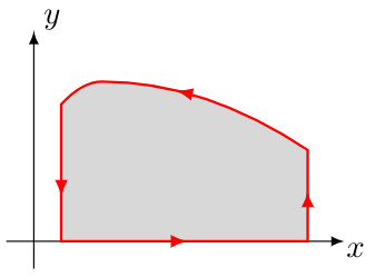
Let’s let that sink in for a second. We can integrate over the region inside a curve boundary merely by doing a related integration around the curve boundary. Imagine counting the cows in a pasture just by walking along the boundary of the pasture and looking at the fence. Or determining the total weight of people in a room by walking along the boundary of the room and listening to them. Bizarre! Somehow the information on the boundary gives you information about the region itself. (Something like this is actually possible with magnetic fields; we can string a long segment of copper wire around the edge of a farmer’s fence and measure the voltage \( V \) between the ends; this voltage \( V = \oint \mathbf{E} \cdot d\mathbf{r} = \iint \nabla \times \mathbf{E} \cdot \mathbf{\hat{n}} \,dS = \iint \frac{\partial\mathbf{B}}{\partial t} \cdot \mathbf{\hat{n}} \,dS \) according to Stokes’s Theorem and Faraday’s Law which states that \( \nabla \times \mathbf{E} = \frac{\partial\mathbf{B}}{\partial t} \). The voltage is equal to the vertical component of the rate of change of magnetic field \( \mathbf{B} \) integrated over the loop area, so we could theoretically eavesdrop over a cell phone conversation inside the fence.)
In the second case of \( \int x\,dy \) we have \( P = 0, Q = x \), so
$$ \oint_C x\,dy = \int\!\!\!\int_R \left({\partial Q\over \partial x}\right) \,dA = \int\!\!\!\int_R \,dA. $$
Integrating \( \int -y\,dx \) and \( \int x\,dy \) aren’t the only two options; Green’s theorem tells us that we can find any twice-differentiable function \( g(x,y) \) and use \( P = \frac{\partial g}{\partial x} \) and \( Q = x + \frac{\partial g}{\partial y} \), because when we plug it into the area integral \( \frac{\partial Q}{\partial x} - \frac{\partial P}{\partial y} \) the \( g \) terms will cancel out.
One that is probably the most appropriate would be \( g = -\frac{1}{2}xy \) which then yields \( \int \frac{1}{2}(x\,dy - y\,dx) \), which when discretized, instead of trapezoids, we end up measuring the area of triangles swept out around the origin;
$$\begin{aligned} S[n] &= S[n-1] + \tfrac{1}{2}\left( x[n] \Delta y - y[n] \Delta x \right) \cr &= S[n-1] + \tfrac{1}{2}\left( x[n] (y[n]-y[n-1]) - y[n] (x[n]-x[n-1])\right) \cr &= S[n-1] + \tfrac{1}{2}(y[n]x[n-1] - x[n]y[n-1]) \end{aligned}$$
You’ll note that this looks nice and smooth, at least for noiseless perfect data.
So here’s our algorithm:
S[n] = S[n-1] + (x[n-1]*y[n] - x[n]*y[n-1])/2.0
Or skip the divide by two and you get twice the area:
S[n] = S[n-1] + x[n-1]*y[n] - x[n]*y[n-1]
The above approach works well with integer math; if using floating-point, it is probably better to avoid subtracting two large quantities of similar magnitude, and instead use the differential form:
S[n] = S[n-1] + (x[n]*(y[n]-y[n-1]) - y[n]*(x[n]-x[n-1])) / 2.0
with or without the 2.0.
Let’s look at some data with Python, where
$$ \begin{align} x_0 &= A_{sig} \cos 2\pi ft +A_{ran} n_x(t)\cr y_0 &= A_{sig} \sin 2\pi ft +A_{ran} n_y(t)\cr \end{align}$$
where \( n_x \) and \( n_y \) are independent unit-amplitude Gaussian white noise waveforms. We’ll also try to filter out the noise:
import numpy as np
import matplotlib.pyplot as plt
import scipy.signal
%matplotlib inline

def filter(x, alpha):
    return scipy.signal.lfilter([alpha],[1,alpha-1],x,zi=x[0:1])[0]

def rancloud(Asig, Aran, f=1, tmax=1, dt = 0.00005, return_all=False, seed=None):
    R = np.random.RandomState(seed)
    t = np.arange(0,tmax,dt)
    x0 = Asig*np.cos(2*np.pi*f*t)
    x = x0 + Aran*R.randn(*t.shape)
    y0 = Asig*np.sin(2*np.pi*f*t)
    y = y0 + Aran*R.randn(*t.shape)
    if return_all:
        return t,x0,x,y0,y
    else:
        return x,y

def cloudplot(Asig, Aran, f=1, tmax=1, dt = 0.00005, alpha=0.01, seed=None):
    t,x0,x,y0,y = rancloud(Asig,Aran,f,tmax,dt,return_all=True, seed=seed)

    fig = plt.figure()
    ax = fig.add_subplot(1,1,1)
    ax.plot(x,y,'.')
    ax.plot(x0,y0,'--r')
    ax.plot(filter(x,alpha),filter(y,alpha),'-k')
    ax.set_aspect('equal')

cloudplot(Asig=1.0, Aran=0.1,f=1,alpha=0.02,dt=1e-5,seed=123)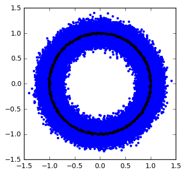
It’s a noise donut! Or a noise bagel, however you prefer. The frequency \( f \) is low enough that with a 20dB signal-to-noise ratio (10x amplitude) we can easily filter out noise and leave ourselves with a very small residual noise content. Somewhere under that black circular-ish trajectory is a red circle representing the signal without noise.
Here’s a noise bialy with 0dB signal-to-noise ratio (1:1 amplitudes):
cloudplot(Asig=1.0, Aran=1.0,f=1,alpha=0.02,dt=1e-5,seed=123)
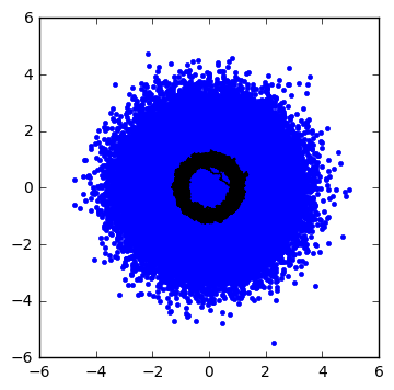
The filter sort of works… now let’s bump up the frequency \( f \) by a factor of 1000:
cloudplot(Asig=1.0, Aran=1.0,f=1000,alpha=0.02,dt=1e-5,seed=123)
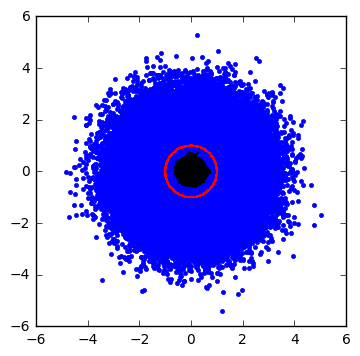
Uh oh, now we have much more trouble separating the noise without filtering out some of the signal content. The filtered signal is a black blob that’s attenuated when compared to the noiseless red circle.
Now let’s try out our swept-area algorithm, first on a signal with no noise. The functions sweptarea_simple and sweptarea_simple_2 use a for-loop and are fairly easy to understand, whereas sweptarea uses the numpy library to perform a vectorized sum.
def sweptarea_simple(x,y):
    assert x.shape == y.shape
    A = np.zeros(x.shape)
    for k in xrange(1, x.size):
        dx = x[k] - x[k-1]
        dy = y[k] - y[k-1]
        A[k] = A[k-1] + x[k]*dy - y[k]*dx
    return A/2.0

def sweptarea_simple_2(x,y):
    assert x.shape == y.shape
    A = np.zeros(x.shape)
    for k in xrange(1, x.size):
        A[k] = A[k-1] + y[k]*x[k-1] - x[k]*y[k-1]
    return A/2.0

def sweptarea(x,y):
    return np.hstack([0,np.cumsum(x[:-1]*y[1:] - x[1:]*y[:-1]) / 2.0])
x,y=rancloud(Asig=1, Aran=0,f=1,dt=1e-5,seed=123) plt.plot(sweptarea(x,y))
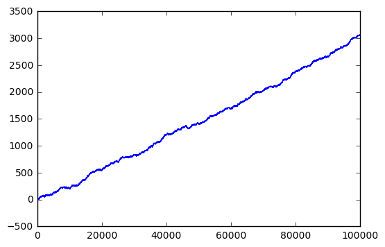
Perfect, we ramp up from 0 to \( \pi \). Now let’s add some noise with amplitude 0.1:
x,y=rancloud(Asig=1, Aran=0.1,f=1,dt=1e-5,seed=123)
plt.plot(sweptarea(x,y))
Hmm. Not great but not bad. What about noise with amplitude 0.05:
x,y=rancloud(Asig=1, Aran=0.05,f=1,dt=1e-5,seed=123)
plt.plot(sweptarea(x,y))
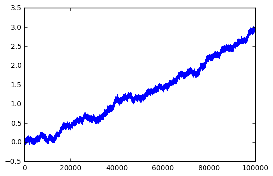
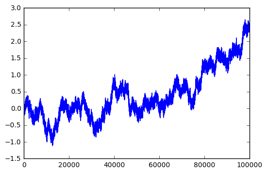
Better. There must be some relationship between the way this algorithm interacts with signal and noise. Let’s look at higher frequency signals and 0dB (1:1) signal-to-noise ratio:
x,y=rancloud(Asig=1, Aran=1,f=1000,dt=1e-5,seed=123)
plt.plot(sweptarea(x,y))
Wow! That’s 0dB signal to noise, and yet we are able to pick up a relatively clean ramp waveform over time.
Let’s think about this for a second. If we have a pair of coordinates \( (x,y) \) that form a circular trajectory of amplitude \( A_{sig} \) and frequency \( f \), then in a given amount of time \( t \) it sweeps out a total area of \( \pi A_{sig}{}^2ft \); the value \( ft \) measures how many complete (or fractional) rotations there are, and \( \pi A_{sig}{}^2 \) is the area of each rotation. Since we are using discrete samples, as long as the sampling rate is significantly faster than the rotation rate, then we’ll come close to a circular trajectory; if the sampling period is \( \Delta t \) then the angle swept out by our signal is \( 2\pi f\Delta t \) and we sample \( n = \frac{1}{f\Delta t} \) points per circle. With \( n=4 \) the area swept out per cycle is a square of side \( \sqrt{2}A_{sig} \), which has area \( 2A_{sig}{}^2 \); the exact answer for integer \( n \) is an area of
$$A_{sig}{}^2 \frac{n}{2} \sin \frac{2\pi}{n}$$
which approaches \( \pi A_{sig}{}^2 \) as \( n \rightarrow \infty \):
for n in [4,8,16,32,64,128]:
    An = n/2.0*np.sin(2*np.pi/n)
    print "%3d %.6f" % (n, An)
4 2.000000 8 2.828427 16 3.061467 32 3.121445 64 3.136548 128 3.140331
Understanding the effect on white Gaussian noise with amplitude \( r \) is trickier. I won’t handle it on a theoretical basis, but if we use our swept-area algorithm empirically just on the noise itself (no signal) and look at a histogram of the increase in its output \( dA \) on each cycle, we can get an idea of what’s going on:
for r in [1, 0.7071]:
    x,y=rancloud(Asig=0, Aran=r,f=0,dt=1e-6,seed=123)
    A = sweptarea(x,y)
    dA = np.diff(A)
    plt.hist(dA,bins=np.arange(-8,8,0.1),log=True)
    print "amplitude", r
    print "mean", np.mean(dA)
    print "stdev", np.std(dA)
amplitude 1
mean 0.000557886848081
stdev 0.708013514984
amplitude 0.7071
mean 0.000278938073906
stdev 0.353999967642
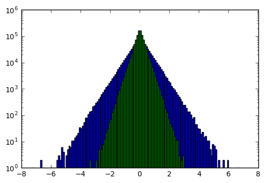
This is an interesting probability distribution; unlike a Gaussian probability distribution function (PDF), which would show up on a log graph as a parabola, it roughly approximates a Laplace distribution with standard deviation \( \sigma = \frac{1}{\sqrt{2}}r^2 \). This has a PDF of
$$\frac{1}{\sqrt{2}\sigma}e^{-\sqrt{2}|x|/\sigma} = \frac{1}{r^2}e^{-2|x|/r^2}$$
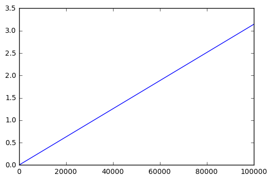
Although the samples of incremental area \( dA \) are not independent (each depends on a pair of noise values, so the \( dA \) values overlap), it does look as though they are uncorrelated, and the area \( A[n] \) approximates a random walk with a variance that increases linearly as \( n\sigma^2 = \frac{n}{2}r^4 \), or a standard deviation that increases as the square root of the number of samples, \( \sqrt\frac{n}{2}r^2 \):
# warning, this takes a while to run; we're going to simulate 10000 different runs
# of a million points each: 10 billion samples!
m = 10000
Asamp = []
for k in xrange(1000):
    x,y=rancloud(Asig=0, Aran=1,f=1000,dt=1e-6,seed=k)
    A = sweptarea(x,y)
    Asamp.append(A[::m].copy())
Asamp = np.vstack(Asamp)
k = np.arange(1e6/m)*m
plt.plot(k,Asamp.std(axis=0))
plt.plot(k,np.sqrt(k)/np.sqrt(2))
plt.xlabel('sample number $k$')
plt.ylabel('standard deviation of 1000 runs')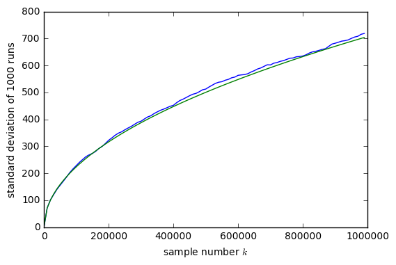
So essentially we are comparing two areas:
- Signal: deterministic signal \( A_{sig}{}^2 ft \frac{n}{2} \sin \frac{2\pi}{n} \approx \pi A_{sig}{}^2 ft = \pi A_{sig}{}^2 fk\Delta t \) where \( n = \frac{1}{f\Delta t} \) sample points per cycle
- Noise: an accumulated random signal with standard deviation at the \( k \)th sample of approximately \( \sqrt{\frac{k}{2}}A_{ran}{}^2 \)
The magnitude of the signal goes up linearly with the number of samples, whereas the magnitude of the noise goes up with the square root of the number of samples. So we can always get a good signal if we are willing to wait long enough.
If we’re looking for some factor \( \lambda = \frac{\mathrm{signal}}{\sigma_{\mathrm{noise}}} \) then this tells us the number of samples \( k \) required to achieve it:
$$ \lambda = \frac{\pi A_{sig}{}^2 fk\Delta t}{\sqrt{\frac{k}{2}}A_{ran}{}^2} = \sqrt{2k}\pi\frac{A_{sig}{}^2}{A_{ran}{}^2} f\Delta t $$
or, in terms of number of samples \( k \):
$$ k = \frac{1}{2}\left(\frac{\lambda A_{ran}{}^2}{\pi A_{sig}{}^2 f\Delta t}\right)^2 $$
So, for example, we could achieve \( \lambda = 20 \) with \( k \Delta t = \) 1 second worth of data with
- \( A_{ran} = 0.02650,\ A_{sig} = 1.0,\ f=1,\ \Delta t = 10^{-5} \)
- \( A_{ran} = 0.04713,\ A_{sig} = 1.0,\ f=1,\ \Delta t = 10^{-4} \)
- \( A_{ran} = 0.08381,\ A_{sig} = 1.0,\ f=1,\ \Delta t = 10^{-3} \)
- \( A_{ran} = 0.14904,\ A_{sig} = 1.0,\ f=10,\ \Delta t = 10^{-4} \)
- \( A_{ran} = 0.26504,\ A_{sig} = 1.0,\ f=10,\ \Delta t = 10^{-3} \)
- \( A_{ran} = 1.18531,\ A_{sig} = 1.0,\ f=100,\ \Delta t = 10^{-3} \)
and if we plot 100 runs of each of these, we can see similar effects in all of them: (for the last one, since there are only 10 points per cycle, we need to take the \( \frac{n}{2} \sin \frac{2\pi}{n} \) factor into account)
fig = plt.figure(figsize=(6.8,16))
Asig = 1
lamb = 20
maxstdev = 4
yrange = 1.0*maxstdev/lamb
parameters = [
    (0.02650, 1.0, 1e-5, 1),
    (0.04713, 1.0, 1e-4, 1),
    (0.08381, 1.0, 1e-3, 1),
    (0.14904, 10.0, 1e-4, 1),
    (0.26504, 10.0, 1e-3, 1),
    (0.83814, 100.0, 1e-3, 1)
]
naxis = 0
naxes = len(parameters)
for Aran, f, dt, T in parameters:
    naxis += 1
    ax = fig.add_subplot(naxes,1,naxis)
    k = None
    for seed in xrange(100):
        x,y=rancloud(Asig=Asig, Aran=Aran,f=f,dt=dt,tmax=T,seed=seed)
        if k is None:
            k = len(x)
            n = 1.0/f/dt
            A_expected_per_cycle = n/2*np.sin(2*np.pi/n)* Asig**2
            A_expected = A_expected_per_cycle * f * (k*dt)

            # Plot curves showing nstdev standard deviations
            krange = np.arange(k)
            t = krange*dt
            normalized_expected_stdev = np.sqrt(krange/2)*Aran**2/A_expected
            for nstdev in xrange(-maxstdev,maxstdev+1):
                ax.plot(t,normalized_expected_stdev*nstdev,'--k',dashes=(5, 4),linewidth=0.4)
        ax.plot(t,sweptarea(x,y)/A_expected - t/T)
    if naxis == naxes:
        ax.set_xlabel('time (seconds)')
    else:
        ax.tick_params(labelbottom='off')
    ax.set_ylim([-yrange,yrange])
    ax.set_ylabel('E')
    title = 'Aran=%f, f=%f, dt=%g, T=%f' % (Aran,f,dt,T)
    if naxis == 1:
        title = 'E = Swept area detected, as a fraction of expected, minus the nominal noiseless signal\n' + title
    ax.set_title(title, fontsize=9)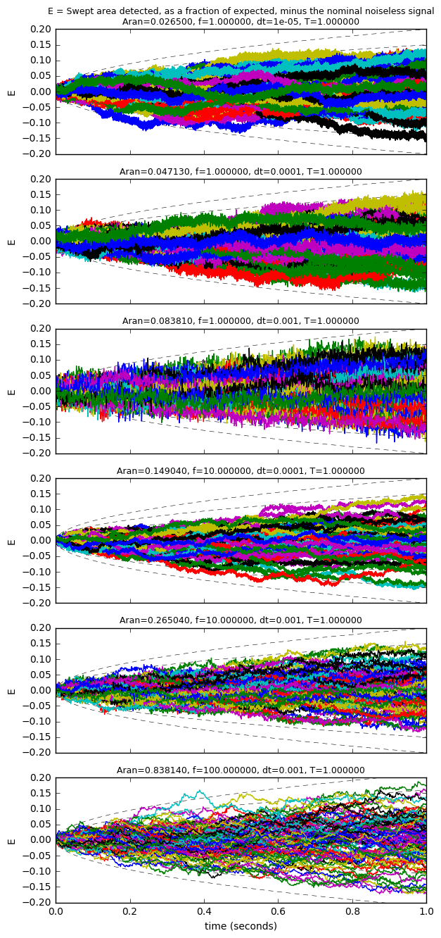
The dashed curves are showing \( N \) standard deviations, from \( N=-4 \) to \( N=4 \); in most cases, the detected signals stray from their expected values by at most about 3-4 standard deviations.
One interesting thing here is that for the same signal parameters (\( A_{sig},\ f \)) and total time, we can tolerate higher noise amplitude if we sample less often, not more, as long as we have some reasonable minimum number (8-12) of samples per cycle of the signal we’re trying to detect. This is because the swept area of the signal is about the same, whether we have 10 samples or 100 or 1000 per cycle, whereas a higher number of samples allows more noise into our detected area. (This algorithm is one of many digital signal processing algorithms where there should be a good match between the sampling rate and the dynamics of the expected signals; for example, low-pass filters and proportional-integral controllers both suffer overflow and resolution problems when using fixed-point calculations, if the sampling rates are too slow or too fast.)
Alternatively, we can use a higher sampling rate, but prefilter the signals to attenuate noise containing significant frequency content above the frequency of the signal we’re trying to detect.
The nice thing about this algorithm is that it works for distorted trajectories in the x-y plane (doesn’t have to be a circle). It also works with trajectories that have an unknown slowly-varying offset; in that case, if the offset is significant, the content of the integrator will have some oscillation, but the net area swept out per cycle is still the same. In this case we have three quantities we need to compare:
- Signal: \( \approx \pi A_xA_yfk\Delta t\cos\phi \) which increases linearly with time (\( A_x \) and \( A_y \) are the separate gains from signals X and Y; \( \phi \) is the phase angle offset from a perfect 90° offset between the signals)
- Noise: an accumulated random signal with standard deviation at the \( k \)th sample of approximately \( \sqrt{\frac{k}{2}}A_{ran}{}^2 \)
- Oscillation: a sinusoidal signal with amplitude \( \approx \frac{1}{2}\sqrt{A_xA_y(b_x{}^2 + b_y{}^2)} \) where \( b_x \) and \( b_y \) are the offsets of each signal — this only holds true if \( A_x \approx A_y \) and \( \phi \approx 0 \), otherwise there are additional oscillatory terms.
The threshold for detecting a valid rotation signal should be set such that the signal is at least 4 or 5 times the noise standard deviation, and at least a few times the amplitude of oscillation.
Here’s a full interactive example (which you can view in its own page) where you can change different settings:
Positive swept areas are shaded green and negative swept areas are shaded red.
The sliders allow you to change these values:
- \( A \) — signal amplitude
- \( A_{ran} \) — noise amplitude
- \( \omega \) — signal frequency
- \( \alpha \) — alters the function used for Green’s Theorem:
- \( \alpha=0 \): circular integration (preferred)
- \( \alpha=1 \): integration along the x-axis
- \( \alpha=-1 \): integration along the y-axis
- \( \phi \) — phase offset from perfect quadrature
If you click “Recenter” and then click a point near the circle, it will change the integration offset so you can see what effect it has.
Have fun exploring!
Wrapup
We looked at a simple signal processing algorithm that measures the swept area integrated over time:
S[n] = S[n-1] + (x[n]*(y[n]-y[n-1]) - y[n]*(x[n]-x[n-1])) / 2.0
or, equivalently stated:
S[n] = S[n-1] + (x[n-1]*y[n] - x[n]*y[n-1])/2.0
Of these two forms, the first is better for floating-point numbers (because it is less susceptible to accumulation of roundoff error) and the second is better for integer or fixed-point calculations because it’s simpler… and usually the factor of 2 can be dropped.
For a repeating trajectory in the \( xy \)-plane with nonzero area, \( S[n] \) will eventually increase (or decrease) to a large number, despite oscillations caused by noise or unknown slowly-varying offset, and it can be used to detect the presence of such a repeating trajectory.
The algorithm essentially derives from Green’s Theorem or Stokes’s Theorem, which integrates a vector field \( \mathbf{F} \) along a closed loop and says that the line integral of the field is equal to the area integral of the curl \( \nabla \times \mathbf{F} \). In this case we use \( \mathbf{F} = \frac{1}{2}\left(x\mathbf{\hat{y}} - y\mathbf{\hat{x}} \right) \) which has a curl of uniform magnitude 1 along the z-axis, so the line integral will give us the area enclosed within the loop… and the rest is just signal processing. Ignore the vector calculus if it makes you nauseous, otherwise, let it sit in your mind… a little cryptic math is good for you every now and then.
© 2017 Jason M. Sachs, all rights reserved.


- Comments
- Write a Comment Select to add a comment
I haven't touched vector calculus in 30 years, but this is interesting none the less. Thank you for taking the time to make this.
Thanks for a wonderful blog, Jason. Can you give me a semester or two to figure what it means?
Thanks for this great article.
Just wanted to add that the swept area formula
(x[n]*(y[n]-y[n-1]) - y[n]*(x[n]-x[n-1])
is an approximation to the instantaneous phase difference (= instantaneous frequency) of the signal. There is a derivation of this formula with simpler math in the Richard Lions DSP trick on "frequency demodulation algorithms"
So, when we are dealing with normalized signals (magnitude = 1), the concept of "swept area" is the same as "instantaneous phase". The article mentions this briefly but I just wanted to highlight.
Thanks again.
To post reply to a comment, click on the 'reply' button attached to each comment. To post a new comment (not a reply to a comment) check out the 'Write a Comment' tab at the top of the comments.
Please login (on the right) if you already have an account on this platform.
Otherwise, please use this form to register (free) an join one of the largest online community for Electrical/Embedded/DSP/FPGA/ML engineers:


