


Ten Little Algorithms, Part 3: Welford's Method (and Friends)
Other articles in this series:
- Part 1: Russian Peasant Multiplication
- Part 2: The Single-Pole Low-Pass Filter
- Part 4: Topological Sort
- Part 5: Quadratic Extremum Interpolation and Chandrupatla's Method
- Part 6: Green’s Theorem and Swept-Area Detection
Last time we talked about a low-pass filter, and we saw that a one-line algorithm could filter out high-frequency noise, and let through the low-frequency components of a signal we were interested in.
This time I’m going to talk about statistics, and the ideas of variance and standard deviation, specifically something called Welford’s method, which gives you accurate estimates of mean and variance without having to keep a bunch of data in memory. I’m also going to show you a modified version of this method that can be used to keep an ongoing estimate of the variance of the most recent history of a signal.
The idea of a signal’s average value, or low-pass filtered value, is pretty easy to get your head around. We just want to smooth out the noise in an unbiased manner, namely come up with an estimated signal so that the signal’s in the middle of the noise. A linear-time invariant low-pass filter will do this; essentially, the error between the noisy signal and the estimate averages out over time. OK, so maybe you need a picture again:
import matplotlib.pyplot as plt
import numpy as np
np.random.seed(123456789)   # repeatable results

f0 = 2
t = np.arange(0,1.0,1.0/65536)
mysignal = (np.mod(f0*t,1) < 0.5)*2.0-1
mynoise = 0.2*np.random.randn(*mysignal.shape)

def lpf(x, alpha, x0 = None):
    y = np.zeros_like(x)
    yk = x[0] if x0 is None else x0
    for k in xrange(len(y)):
        yk += alpha * (x[k]-yk)
        y[k] = yk
    return y

delta_t = t[1]-t[0]
tau = 0.003
alpha = delta_t/tau
mysignal_estimate = lpf(mysignal+mynoise, alpha, 0)

plt.figure(figsize=(8,6))
plt.plot(t, mysignal+mynoise, '#e0e0e0',
         t, mysignal_estimate,'green')
plt.plot(t, mysignal, ':', color='black')
plt.legend(('signal + noise','estimated signal','original signal'),loc='lower left', fontsize=10)
plt.ylim(-1.8,1.8);
Here we were able to recover the low frequencies of the original signal while rejecting frequencies with a cutoff of around \( f_c = \frac{1}{2\pi\tau} \approx 53 \) Hz. The estimated signal has a little bit of phase lag compared to the original signal, but not much, and the noise is attenuated greatly.
Now, the question becomes: what if we don’t care about the signal, but we want to know something about the noise?
In particular: how much noise is present?
Let’s look at a simpler case, where we just take the first 0.2 seconds of the signal + noise:
y1 = (mysignal+mynoise)[t<0.2]
t1 = t[t<0.2]
plt.plot(t1,y1)
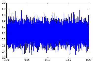
This essentially looks like a constant signal with a constant amount of noise. The term “constant amount of noise” isn’t really precise; instead, we can say that the noise is produced by a stationary process, which essentially means its probability distribution, frequency spectrum, cross-correlation, and other statistical metrics don’t change over time. If we make that assumption (constant signal, noise coming from a stationary process), statistics can help us come up with the best estimate of the signal and noise characteristics.
The sample mean value \( \bar{x} \) is defined precisely as
$$ \bar{x} = \frac{1}{N}\sum_{k=0}^{n-1}{x_k}$$
which essentially means we just take N samples, sum them up, and divide by N. It’s just the arithmetic average.
The sample variance \( s^2_{x} \) is also defined precisely as
$$ s^2_{x} = \frac{1}{N-1}\sum_{k=0}^{n-1}{(x_k - \bar{x})^2}$$
This is a little more complicated, but we essentially just sum up the squared differences between each sample value and the mean value, and divide by \( N-1 \). The reason for the \( N-1 \) vs. \( N \) is subtle, and you can read about it in the Wikipedia article on Bessel’s correction.
In any case, what this sample variance \( s^2_{x} \) is giving us is an estimate of the actual variance \( \sigma^2_x \), which is the expected value of the squared difference between individual sample points and the mean. Blah blah blah. Too much math. Okay, let’s just try it with numpy.
print "sample mean:         ", np.mean(y1)
print "sample variance:     ", np.var(y1)
print "sample std deviation:", np.std(y1)
sample mean:          1.00056783436
sample variance:      0.0397044481571
sample std deviation: 0.199259750469
Note that the sample mean is around 1.000 and the sample standard deviation \( s_x \), which is just the square root of the sample variance, is around 0.200. These are the numbers we put in to generate the signal in the first place. The numpy.random.randn() function gives out random numbers with a Gaussian distribution, a mean of zero, and a standard deviation of 1.0. If you want numbers with a standard deviation of K, you just multiply the results from randn() by K.
The sample mean and sample variance are themselves random variables, and although you can expect to get numbers near the actual mean and variance, they’re always a little bit off. If you care about how much this is numerically, you can look up the variance of the sample mean and variance and see that they both scale as \( \approx \frac{1}{\sqrt{N}} \) — if you want to cut your expected error by half, you have to take four times as many number of samples.
In any case, if the number of samples is fixed, the sample mean and variance will give you the best estimates of the actual (population) mean and variance.
So let’s say you’re designing a DMM, and you measure resistance by putting a calibrated current through an unknown value, then measuring a bunch of voltage samples. You could estimate the resistance itself by taking the mean value of those voltage samples, divided by the calibrated current, and then compute the standard deviation, which will tell you something about how noisy your measurements are.
Batch vs. stream processing
One of the major issues (especially with embedded systems, where RAM tends to be much more scarce than on a PC) with the sample mean and variance formulas, is that the straightforward evaluation of these formulas requires you to keep an entire batch of samples in memory and then run a bunch of computations on that whole batch. If I’m taking 100,000 samples a second and I want to average over 10 seconds of data, that’s a million samples! While most microcontrollers with ADCs can digitize at this speed very easily, storing a million samples of, say, 16-bit data requires 2Mbytes of RAM. But my dsPIC33EP256MC506 only has 48K RAM, and I need some of it for other purposes. Even if we did have room to store it all, once we take the samples of data we still have to wait to run the calculations.
So what’s better is stream processing, where you run the calculations as the data comes in, and don’t keep around past data any more than you need to.
The sample mean value is pretty simple to evaluate with stream processing. Just keep a running sum of the data and keep track of the number of samples:
S += x;
++n;
(or \( S[n] = S[n-1] + x[n] \) as my signal-processing friends like to see)
Then, whenever you want to know what the mean value is, you can just compute S/n, whether it’s at the very end, or somewhere in the middle of your data where you want to see how things are progressing.
The sample variance is a little more difficult. What Wikipedia calls the naïve algorithm requires you to keep both a running sum and a running sum of squares:
S += x;
S2 += x*x;
++n
And when you want to know the sample variance, you just compute
v = (S2 - (S*S)/n)/(n-1);
and take the square root if you want sample standard deviation. The problem is that this algorithm plays badly with floating-point precision. Let’s take a look and give it a try.
def naive_stats(x_collection):
    S = 0
    S2 = 0
    n = 0
    for x in x_collection:
        S += x
        S2 += x*x
        n += 1
    m = S/n
    v = (S2 - (S*S)/n)/(n-1)
    return m,v

naive_stats(y1)
You’ll notice that the mean is spot-on, and the sample variance is really close to what numpy.var() calculated (0.03970748 vs. 0.03970444).
Now let’s add a larger signal; instead of a mean value of 1.0, we’ll add in 9999 to get a mean value of 10000:
y1b = y1 + 9999

print "naive_stats:", naive_stats(y1b)
print "numpy:      ", (np.mean(y1b), np.var(y1b))
naive_stats: (10000.000567834355, 0.039707283083466847)
numpy:       (10000.000567834355, 0.039704448157095722)
Hmm, a little worse here. What if we had a mean value of 1000000?
y1b = y1 + 999999

print "naive_stats:", naive_stats(y1b)
print "numpy:      ", (np.mean(y1b), np.var(y1b))
naive_stats: (1000000.000567832, 0.048065918974593731)
numpy:       (1000000.0005678344, 0.039704448157135086)
Uh oh. That doesn’t look too good. How about 107 or -107?
for A in [1e7, -1e7]:
    y1b = y1 - 1 + A
    print "naive_stats:", naive_stats(y1b)
    print "numpy:      ", (np.mean(y1b), np.var(y1b))
naive_stats: (10000000.000567846, 0.17578393224994279) numpy: (10000000.000567835, 0.039704448154261794) naive_stats: (-9999999.999432154, -0.097657740138857099) numpy: (-9999999.9994321652, 0.039704448154261794)
Completely bonkers. We even get a negative variance if we’re not careful, which makes no sense and will give you an error when you take the square root.
The problem here is that when we do this calculation:
(S2 - (S*S)/n)
we are subtracting two very large numbers if the standard deviation is much smaller than the mean, and that is a recipe for poor precision.
At this point we should pull out our copy of Donald Knuth’s The Art of Computer Programming, Volume 2: Seminumerical Algorithms and turn to the section on floating-point arithmetic:

Those funny symbols \( \oplus \ominus \otimes \oslash \) are just there to designate the approximation operations of floating-point machine arithmetic, as opposed to the exact mathematical operators \( + - \times / \); when it comes to computations in floating-point, the computer is almost always inaccurate, even if the error is very small. Rewritten in “normal” discrete-time math for clarity, our algorithm is this:
$$\begin{eqnarray} M[k] &=& M[k-1] + \frac{1}{k}\left(x[k] - M[k-1]\right) \cr S[k] &=& S[k-1] + \left(x[k]-M[k-1]\right)\left(x[k]-M[k]\right) \end{eqnarray}$$
We can write Welford’s method in Python as follows:
def welford0(x_array):
    k = 0
    for x in x_array:
        k += 1
        if k == 1:
            M = x
            S = 0
        else:
            Mnext = M + (x - M) / k
            S = S + (x - M)*(x - Mnext)
            M = Mnext
    return (M, S/(k-1))

for A in [1e7, -1e7]:
    y1b = y1 - 1 + A
    print "welford0:", welford0(y1b)
    print "numpy:   ", (np.mean(y1b), np.var(y1b))
welford0: (10000000.000567824, 0.039707477399781213) numpy: (10000000.000567835, 0.039704448154261794) welford0: (-9999999.9994321764, 0.039707477399781213) numpy: (-9999999.9994321652, 0.039704448154261794)
which is much better, but still slightly off in variance… so we have to wonder if maybe the numpy.var() method uses the \( N \) divisor rather than \( N-1 \). Sure enough, looking closely at the documentation of numpy.var(), it has a ddof which represents the number of degrees of freedom to be subtracted, and the notes say
In standard statistical practice,
ddof=1provides an unbiased estimator of the variance of a hypothetical infinite population.
So let’s fix it:
for A in [1e7, -1e7]:
    y1b = y1 - 1 + A
    print "welford0:", welford0(y1b)
    print "numpy:   ", (np.mean(y1b), np.var(y1b, ddof=1))
welford0: (10000000.000567824, 0.039707477399781213) numpy: (10000000.000567835, 0.039707477409480704) welford0: (-9999999.9994321764, 0.039707477399781213) numpy: (-9999999.9994321652, 0.039707477409480704)
Hey, that’s much better. One of the things I’ve noticed is that you don’t have to handle the first case separately; you can just initialize the variables outside the loop to zero, so that the first time through we will calculate
 Mnext = 0 + (x - 0) / 1          = x
 S = 0 + (x - 0) * (x - Mnext)    = 0
and, yeah, it’s an “extra” calculation, but it also lets you just blindly loop through the whole array without having to special-case the first iteration.
def welford(x_array):
    k = 0
    M = 0
    S = 0
    for x in x_array:
        k += 1
        Mnext = M + (x - M) / k
        S = S + (x - M)*(x - Mnext)
        M = Mnext
    return (M, S/(k-1))

for A in [1e7, -1e7]:
    y1b = y1 - 1 + A
    print "welford:", welford(y1b)
    print "numpy:   ", (np.mean(y1b), np.var(y1b, ddof=1))
welford: (10000000.000567824, 0.039707477399781213) numpy: (10000000.000567835, 0.039707477409480704) welford: (-9999999.9994321764, 0.039707477399781213) numpy: (-9999999.9994321652, 0.039707477409480704)
Same results. Quick and simple. So that’s Welford’s method.
Like many statistical methods, it is more accurate if you can normalize the inputs, namely subtract off a gross estimate of the mean, and then scale by a gross estimate of standard deviation, leaving you with a normalized input \( x’ \) which has a mean closer to zero and a standard deviation closer to 1.0:
$$ x’ = \frac{x-\mu_0}{\sigma_0} $$
But for typical applications with 16-bit inputs, you can probably get away without bothering to normalize.
Variations on a theme: Nonstationary processes, non-constant data, and real-time estimates of noise amplitude
Things get more interesting if we have noise that is nonstationary. Here’s an example of that:
np.random.seed(123456789)   # repeatable results

f0 = 2
t = np.arange(0,1.0,1.0/65536)
mysignal0  = (np.mod(f0*t,1) < 0.5)*2.0-1
mysignal1 = lpf(mysignal0, 0.005)

def ratelimit(x,maxdelta):
    y = np.zeros_like(x)
    yi = x[0]
    for i,xi in enumerate(x):
        delta = xi - yi
        yi += max(-maxdelta, min(maxdelta, delta))
        y[i] = yi
    return y

mytrapz = ratelimit(mysignal0, 0.01)
modulator = ((np.mod(f0*t+0.25,1) < 0.5)*0.5+0.5) * 0.04
mynoise = modulator * np.random.randn(*mysignal0.shape)

fig=plt.figure(figsize=(8,6))
ax=fig.add_subplot(2,1,1)
ax.plot(t,mysignal1+mynoise,'gray',t,mysignal1,'--k')
ax.legend(('signal+noise','signal'),loc='lower left')
ax=fig.add_subplot(2,1,2)
ax.plot(t,mynoise,'gray',t,modulator,'--k')
ax.set_ylabel('noise')
Here the noise amplitude is modulated by a square wave, with amplitude switching back and forth from 0.02 to 0.04. What if we wanted to see how the noise amplitude looks over time?
We can take a clue from Welford’s method and try to turn it into a filter rather than just a single statistic:
def statfilt(x_array, alpha, beta=None, x0=None):
    m = np.zeros_like(x_array)
    S = np.zeros_like(x_array)
    Sk = 0
    beta = alpha if beta is None else beta
    mk = x_array[0] if x0 is None else x0
    for k, x in enumerate(x_array):
        mnext = mk + alpha*(x-mk)
        Sk = Sk + beta*((x-mk)*(x-mnext) - Sk)
        mk = mnext
        m[k] = mk
        S[k] = Sk
    return m, np.sqrt(S)

tau1 = 0.0002
tau2 = 0.03
delta_t = t[1]-t[0]
m, stdev = statfilt(mysignal1+mynoise, alpha=delta_t/tau1, beta=delta_t/tau2)

fig=plt.figure(figsize=(8,6))
ax=fig.add_subplot(3,1,1)
ax.plot(t,mysignal1+mynoise,'gray',t,mysignal1,'--k')
ax=fig.add_subplot(3,1,2)
ax.plot(t,m)
ax=fig.add_subplot(3,1,3)
ax.plot(t,stdev,t,modulator)
ax.legend(('estimated','actual'),loc='best',fontsize=10)
ax.set_ylabel('noise amplitude')
ax.grid('on')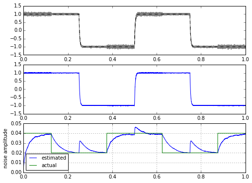
That’s interesting — essentially it looks like we might be able to calculate a filtered variance very easily. The only problem is that we get these glitches when the signal jumps all of a sudden. In fact, I kind of cheated here by using an input signal that was filtered first before adding noise. If I use a trapezoid or a square wave as the input signal, we get much higher glitches in our estimator:
for signal in [mytrapz, mysignal0]:
    m, stdev = statfilt(signal+mynoise, alpha=delta_t/tau1, beta=delta_t/tau2)

    fig=plt.figure(figsize=(8,6))
    ax=fig.add_subplot(3,1,1)
    ax.plot(t,signal+mynoise,'gray',t,signal,'--k')
    ax=fig.add_subplot(3,1,2)
    ax.plot(t,m)
    ax=fig.add_subplot(3,1,3)
    ax.plot(t,stdev,t,modulator,'gray')
    ax.legend(('estimated','actual'),loc='best',fontsize=10)
    ax.set_ylabel('noise amplitude')
    ax.grid('on')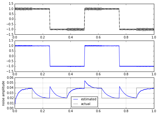
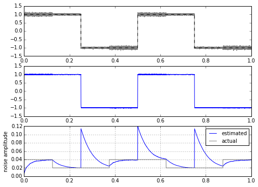
There’s no easy way to get around this problem. It’s caused by the fact that after a step, the filtered version of the step is delayed, so all of a sudden there is a huge difference between input waveform and the filtered version of it — this difference gets added into the noise calculator. Another way of looking at it is in the frequency domain, where we have spectrum overlap between the part of our signal that we consider noise (the high frequency content of the noise), and the part of our signal that isn’t noise (the high frequency content of the square wave edges). We can try to make this a little better, and play tricks with clipping to reject the rate of change of large amplitudes:
def statfilt2(x_array, alpha, beta=None, x0=None, clip1=5.0, clip_eps=1e-5):
    m = np.zeros_like(x_array)
    S = np.zeros_like(x_array)
    Sk = 0
    beta = alpha if beta is None else beta
    mk = x_array[0] if x0 is None else x0
    for k, x in enumerate(x_array):
        mnext = mk + alpha*(x-mk)
        Sk_in = (x-mk)*(x-mnext)
        if Sk_in > Sk:
            Sk_diff = min(Sk_in - Sk, clip1*Sk + clip_eps)
            # limit difference to some multiple "clip1" of the current variance estimate
            # (use something in the 5-10 range since this will catch the vast majority
            # of Gaussian noise content; 3-4 is not enough since that lets some noise
            # slip through, and we will underestimate noise amplitude)
            #
            # (+ a noise floor clip_eps to help us get unstuck in case Sk is ever 0)
        else:
            Sk_diff = Sk_in - Sk
        Sk = Sk + beta*Sk_diff
        mk = mnext
        m[k] = mk
        S[k] = Sk
    return m, np.sqrt(S)

for signal in [mysignal0, mytrapz, mysignal1]:
    m, stdev = statfilt2(signal+mynoise, alpha=delta_t/tau1, beta=delta_t/tau2)

    fig=plt.figure(figsize=(8,6))
    ax=fig.add_subplot(3,1,1)
    ax.plot(t,signal+mynoise,'gray',t,signal,'--k')
    ax=fig.add_subplot(3,1,2)
    ax.plot(t,m)
    ax.set_ylabel('filtered signal m')
    ax=fig.add_subplot(3,1,3)
    ax.plot(t,stdev,t,modulator,'gray')
    ax.legend(('estimated','actual'),loc='best',fontsize=10)
    ax.set_ylabel('noise amplitude')

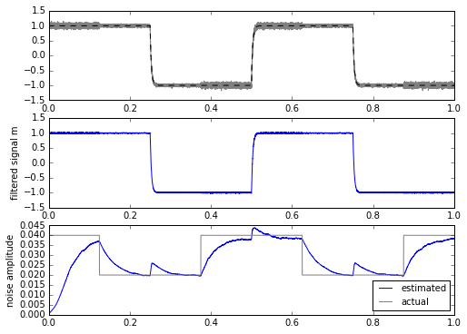
Hmm. Well, this really helps out when the input signal is a square wave, but not as much if it’s a trapezoidal waveform or a low-pass-filtered square wave.
Another approach is to modify the filter: when there are edges, let it react faster than it usually does, by keeping it within a band of \( \pm K s \) of the input, where K is fixed and s is our dynamically-changing estimate of the standard deviation. When the input is closer to the mean, then we filter normally.
def statfilt3(x_array, alpha, beta=None, x0=None, clip1=2.236, clip_eps=1e-10):
    # 2.236 = sqrt(5)
    m = np.zeros_like(x_array)
    S = np.zeros_like(x_array)
    Sk = 0
    beta = alpha if beta is None else beta
    mk = x_array[0] if x0 is None else x0
    for k, x in enumerate(x_array):
        mnext = mk + alpha*(x-mk)
        sk = np.sqrt(Sk)
        band = clip1*sk + clip_eps
        mnext = x + max(-band,min(band,mnext-x))
        Sk = Sk + beta*((x-mk)*(x-mnext) - Sk)
        mk = mnext
        m[k] = mk
        S[k] = Sk
    return m, np.sqrt(S)

for signal in [mysignal0, mytrapz, mysignal1]:
    m, stdev = statfilt3(signal+mynoise, alpha=delta_t/tau1, beta=delta_t/tau2)

    fig=plt.figure(figsize=(8,6))
    ax=fig.add_subplot(3,1,1)
    ax.plot(t,signal+mynoise,'gray',t,signal,'--k')
    ax=fig.add_subplot(3,1,2)
    ax.plot(t,m)
    ax.set_ylabel('filtered signal m')
    ax=fig.add_subplot(3,1,3)
    ax.plot(t,stdev,t,modulator,'gray')
    ax.legend(('estimated','actual'),loc='best',fontsize=10)
    ax.set_ylabel('noise amplitude')

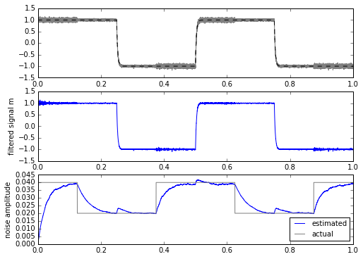
This is a bit more promising. The only drawback is that we have to calculate the square root every time, which is computationally more expensive in most embedded systems. This isn’t a horrible thing, even on a system with fixed-point multiplication and no floating-point: there are approximations for sqrt() for slowly-changing input waveforms that can come close while requiring less computation.
In general, I’m not very fond of these sorts of heuristic algorithm “fixups” — yes, they can improve the performance of simpler, linear methods in some cases, but it’s often hard to test all the edge cases and ensure that your algorithm doesn’t perform poorly in some cases, or even worse, get stuck in some state it can’t get out of.
But if I look the other way and forget about my principles, it looks like we have a noise metric that essentially shows us variation between 0.02 and 0.04. We have an obvious tradeoff between the filtering constants and accuracy: slower filters effectively integrate over a larger period of time, which reduces the variance of the calculation, at the expense of more of a delay in measurement.
Be aware that distinguishing between high-frequency components of a signal step, and high-frequency components of noise, is a very difficult task, and the clipping and fixed-up-filter approaches I used here are both somewhat artificial solutions.
Another possible approach is to use an adaptive filter of some kind, like the Kalman filter, which is good for these sorts of problems, but the matrix math gets heavy, and even a simple 1-D Kalman filter is something I don’t trust myself to implement correctly. Let’s save that one for another day. (And no promises: I have too many other articles that are waiting for me to write them.)
Aside from Kalman filters, dynamic noise estimates don’t seem to be commonly described in signal processing textbooks, so you’ll have to play around with these sorts of algorithms for your situation. I can’t promise this approach is the best.
Wrapup
In any case, Welford’s method gives us a simple streaming (on-line) method for computing sample mean and variance, without having to store large numbers of values. We just update the computations and throw the input data away. We will get the exact answer (well, within a small numerical error band caused by machine precision) that we would have gotten from a batch-processing method using the conventional definition for sample variance. This is much more accurate than the naive method of accumulating sums and accumulating sums of squares, which can be very inaccurate in cases where the mean value is large compared to the standard deviation.
I’ve used a modified version of Welford’s method, more akin to a filter, to provide a continuous estimation of signal variance. It performs well except in cases where the input undergoes sudden jumps; the error caused by this effect can be reduced by some nonlinear techniques.
© 2015 Jason M. Sachs, all rights reserved.


- Comments
- Write a Comment Select to add a comment
I'm wondering a bit about this method still. I would like to have something like this running on a real time embedded system continuously. I guess this one will not do in the long run as you increase a sum every cycle, sooner or later an overflow will occur. Additionally this system is not using floating point variables. Are there any known methods for doing this?


kaz
%%%%%%%%%%%%%%%%%%%%%%%%
[So whats better is stream processing, where you run the calculations as the data comes in, and dont keep around past data any more than you need to.
The sample mean value is pretty simple to evaluate with stream processing. Just keep a running sum of the data and keep track of the number of samples:
S += x;
++n;
(or S[n]=S[n?1]+x[n] as my signal-processing friends like to see)
Then, whenever you want to know what the mean value is, you can just compute S/n, whether its at the very end, or somewhere in the middle of your data where you want to see how things are progressing.].
%%%%%%%%%%%%%%%%%%%%%%%%%%%
I don't get it. You either can do running average or block based average. your description seems combining them. block average only needs counter. running average needs memory for delay units.
either way overflow is avoided by reset or subtraction respectively.
Thanks
Kaz
To post reply to a comment, click on the 'reply' button attached to each comment. To post a new comment (not a reply to a comment) check out the 'Write a Comment' tab at the top of the comments.
Please login (on the right) if you already have an account on this platform.
Otherwise, please use this form to register (free) an join one of the largest online community for Electrical/Embedded/DSP/FPGA/ML engineers:


